Gradient descent III: SGD for Polyak-Łojasiewicz functions

October 2023

In the preceding note on stochastic gradient descent we proved some convergence guarantees for functions satisfying strong convexity assumptions. Now, we move on to a more realistic setting. A differentiable function $f:\mathbb{R}^d \to \mathbb{R}$ is $\eta$-Polyak-Łojasiewicz^[1] ($\eta$-PL for short) if it is bounded below and if for every $x$,

$$f(x) - \inf f \leqslant \frac{1}{2\eta}|\nabla f(x)|^2.$$

What is really impressive is that most results on gradient descent or SGD transfer directly from strongly convex functions to PL functions... but PL functions need not even be convex! This is a great leap forward for optimization, and it's quite a recent finding.

Two important examples of PL functions which are not convex are

• $f(x) = \mathrm{dist}(x,S)^2$ where $S$ is any set and the distance is the euclidean one.

• $f(x) = |F(x) - y|^2$ when $F:\mathbb{R}^d \to \mathbb{R}^d$ and the smallest singular value of the Jacobien $DF(x)$ is uniformly bounded away from zero, ie $\min_x \sigma_{\min}(DF(x))>\mu$. This roughly says that $f$ is locally invertible, and « uniformly so ». In this case $F$ is $\mu$-PL.

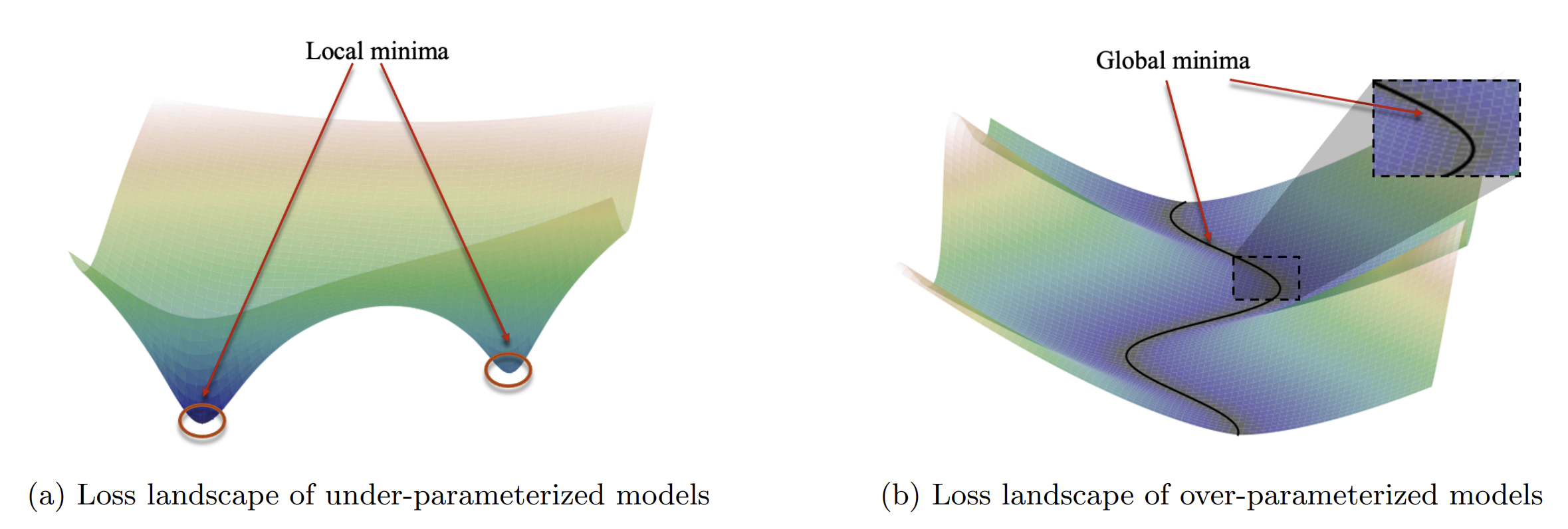
These examples show that PL functions form a really wider class than (strongly) convex functions. On the other hand, they need not have a unique minimizer, which is the case for strongly convex functions. Indeed, (1) implies that any critical point ($\nabla f (x) = 0$) has $f(x) = \inf f$. In other words, local minima are not unique at all, but they are all global, see (b) in the Figure below^[2].

Consequently, optimization algorithms will not find minimizers of $f$ but they will search for the minimum value of $f$ instead. Just as for strongly convex functions, there is a general convergence result for vanilla Gradient Descent, but I'll only present the corresponding result for SGD. That is, we are now in the minimization of a function $f$ assuming the shape

$$f(x) = \frac{1}{n}\sum_{i=1}^m f_i(x)$$

where the $f_i : \mathbb{R}^d \to \mathbb{R}$ are PL functions. The SGD is given by the updates

$$x_{n+1} = x_n - \varepsilon_n \nabla f_{i_n}(x_n)$$

where for each step $n$, the index $i_n$ is independent of $x_n$ and $i_n \sim \mathrm{Unif}\{1,\dotsc, d\}$. For future reference, we recall that $f$ is $M$-smooth if $f(y)-f(x)\leqslant \langle \nabla f(x), y-x\rangle + M/2 |x-y|^2$, see the note on GD.

The difference between this and the classical GD result is the additional term featuring $\delta$. Strikingly, when all the $f_i$ have the same minimal value (ie $\inf f_i = \inf f$), this term disappears since $\delta = 0$. This situation is called interpolation. It does imply that all the $f_i$ can reach their minimal value at the same time. One might be tempted to check how this $\delta$ relates to the local variance $\sigma$ introduced in the case of strongly convex functions. It turns out^[3] that if all the $f_i$ are $M$-smooth, (i) in general, $\sigma \leqslant 2M\delta$; (ii) if the $f_i$ are $\mu$-strongly convex, then $2\mu \delta \leqslant \sigma$. So in the case of strongly convex functions, these two parameters measure the same thing.

Proof

It is once again the same kind of tricks as for GD and SGD, but now we directly apply them to $f(x_n)$ instead of applying them to $x_n$. For simplicity, we will suppose that the minimum value of $f$ is zero, ie $\inf f = 0$.

Writing the fact that $f$ is $M$-smooth (since if all the $f_i$ are $M$-smooth), then using the definition of the SGD update rule, we have

$$\begin{aligned}f(x_{n+1}) - f(x_n) &\leqslant \langle \nabla f(x_n), x_{n+1} - x_n\rangle + \frac{M}{2}|x_{n+1} - x_n|^2 \\ &= - \varepsilon \langle \nabla f (x_n), \nabla f_{i_n}(x_n)\rangle + \frac{M\varepsilon^2}{2}|\nabla f_{i_n}(x_n)|^2. \end{aligned}$$

We now take conditional expectations with respect to $x_n$. Since $\mathbb{E}_n[\nabla f_{i_n}(x)] = \nabla f (x)$, we get

$$f(x_{n+1}) \leqslant f(x_n) - \varepsilon | \nabla f(x_n)|^2 + \frac{M\varepsilon^2}{2}\mathbb{E}_n[|\nabla f_{i_n}(x_n)|^2].$$

Now we need to estimate the latter expectation and for this, we use the following elementary lemma.

The proof is left as an exercise. Incidentally, this fact sheds some light on the PL-condition. In fact, PL functions satisfy the opposite inequality up to a constant. This is why PL functions efficiently replace the strong convexity assumption.

Apply (9) to the $M$-smooth function $f_{i_n}$ to get

$$\begin{aligned}\mathbb{E}_n[|\nabla f_{i_n}(x_n)|^2] &\leqslant 2M \mathbb{E}_n [f_{i_n}(x_n) - \inf f_{i_n}] \\ &= 2M\mathbb{E}_n [f_{i_n}(x_n) - f_{i_n}(x)] + 2M\mathbb{E}_n[f_{i_n}(x) - \inf f_{i_n}] \\ &= 2Mf(x_n) + 2M\delta. \end{aligned}$$

Now, plug these inequalities in (8) to get

$$f(x_{n+1}) \leqslant f(x_n) - \varepsilon | \nabla f(x_n)|^2 + M^2\varepsilon^2 f(x_n) + M^2\varepsilon^2 \delta.$$

We did not use the PL condition – but not for much longer. When reversed, (1) tells us that $-|\nabla f(x_n)|^2 \leqslant -2\eta f(x_n)$. We plug this into the last inequality, reorganize terms, take expectations, and we get

$$\mathbb{E}[f(x_{n+1})] \leqslant (1- 2\eta \varepsilon + M^2\varepsilon^2) \mathbb{E}[f(x_n)] + M^2\varepsilon^2 \delta.$$

It's over now. The first factor is $1 + \varepsilon (M^2\varepsilon - 2\mu)$ and we chose the stepsize $\varepsilon$ precisely so that $M^2\varepsilon - 2\eta < -\eta$. The final recursion reads

$$\mathbb{E}[f(x_{n+1})] \leqslant (1 - \varepsilon \eta)\mathbb{E}[f(x_n)] + (M\varepsilon)^2\delta.$$

This is once again a classical recursion of the form $u_{n+1} \leqslant a u_n + b$ and it is easily leveraged to $u_{n+1}\leqslant b(1 - a^n )/(1-a) + a^n u_0$, hence

$$\mathbb{E}[f(x_{n+1})] \leqslant (1 - \varepsilon \eta)^n f(x_0) + \frac{M^2\varepsilon}{\eta}\delta.$$

Discussion

• Minibatch SGD. In this note and the preceding one I chose the simplest SGD version, the one where $f$ is a sum and we choose one of the functions to estimate the full gradient. The same proof can be adapted to more complicate settings, such as mini-batches where at each step we draw a random batch of indices $\{i_1, \dotsc, i_B\}$ uniformly at random on $[m]$ and estimate the gradient with $\frac{1}{B}\sum_{k=1}^B \nabla f_{i_k}(x)$. The main difference will be on the definition of the discrepancy $\delta$ which needs to be adapted (it's straightforward).

• Noisy SGD. The other variant of SGD is when we have access to a noisy estimate of the gradient, say for simplicity $\nabla f(x) + \xi$ where $\xi$ is an independent small Gaussian noise. I don't know if there are results for this (typically, they shall relate to the mixing time of the Langevin dynamics).

• Local PL functions. The PL assumption is considerably more realistic than strong convexity. PL functions need not be convex and need not have a unique minimizer. However, the absence of non-global local minima can be considered highly unrealistic, especially when dealing with neural networks. One possible workaround would be to replace the global PL condition with local ones. What happens when we only assume that functions are locally PL? Many results were obtained in this line: this one or this one for proximal gradient. More recently this paper by Sourav Chatterjee goes in the same direction. However these results are only valid for classical gradient descent. There are no similar results for SGD.

• Neural Networks. Applying such results to neural networks remains a moot point. The main argument is that the loss landscape for NNs in the infinite width regime (and for certain initializations), the loss landscape is almost quadratic. The paper by Liu, Zhu, Belkin is a wonderful read for anyone interested in the topic. They essentially study the small singular values of the differential of a NN – these singular values are the spectral values of the Neural Tangent Kernel, and the NTK is supposed (under certain circumstances) to be… almost constant. Hence, NNs are almost PL.

References

These three notes on GD and SGD were mostly taken from the wonderful survey by Guillaume Garrigos and Robert Gower, here. Guillaume proofread this note. Most of the remaining errors are due to him.

---

^[1] The Polish Ł is actually pronounced like the French « ou » or the English « w ». So Łojasiewicz sounds like « Wo-ja-see-yeah-vitch ». Among well-known Polish names with this letter, there's also Rafał Latała, Jan Łukasiewicz or my former colleague Bartłomiej Błaszczyszyn whose name is legendarily hard to pronounce for Westerners.

^[2] Figure extracted from the Liu, Zhu, Belkin paper.

^[3] See Lemma 4.18 in the survey.