🏋🏼 Heavy tails IV: cascades of events

June 2026

Sixty stocks jump in the same minute — coincidence or not? In many fields where we study the occurrence of simultaneous events in time, it turns out that the number of simultaneous events is often small, but can also be dramatically big, with a typically heavy-tail distribution. There is a nice explanation for this phenomenon, coming from the theory of random avalanches –- a fancy name for Galton-Watson processes. This post explains the connection.

Price jumps in financial markets
Galton-Watson processes and the total population law
The CLT approximation
You don’t need to be critical to have heavy tails
References

Price jumps in financial markets

ook at the prices of stocks (say, in the S&P500) and examine how many of them experience a jump at the same time (say, within the same hour or minute). This is called co-jump analysis. Here are two plots taken from an insightful paper: 

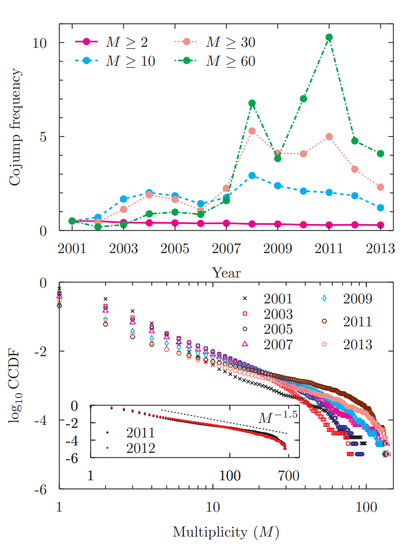
On the top, you see the number of minutes, in every year, where there was a co-jump. For example the green line counts the minutes where more than 60 stocks jumped at the same time. The most interesting plot is the second one, plotting the distribution of the sizes of the co-jumps. The scale is logarithmic, and clearly this distribution looks heavy tailed, perhaps with an index of $\alpha=0.5$ , which would mean that the number $N(k)$ of co-jumps of $k$ stocks is roughly of order $O(k^{-1.5})$ . As we’ll see, other papers estimate the tail to be rather $O(k^{-2})$ .

Why should these types of events exhibit a heavy-tail behaviour? There is a very simple answer: there is a "cascading" happening behind the jumps. One jump occurs somewhere: say, the price of $\textsf{AAPL}$ goes up first. Then this jump triggers a few jumps in related companies, like $\textsf{GOOGL}, \textsf{MSFT}$ . The jump for $\textsf{GOOGL}$ triggers in turn another jump at $\textsf{AMZN}$ . Maybe the jump at Microsoft didnt trigger anything, but in turn the jump at $\textsf{AMZN}$ triggers a jump in $\mathsf{NFLX}$ . And so on, the initial event cascades into the network, until the contagion stops.

This kind of cascading effect (« random avalanches ») naturally leads to a heavy-tailed distribution for the total number of events that happened in the end. This is what we are going to prove.

Galton-Watson processes and the total population law

The total number of events in a cascade described as earlier is well captured by Galton-Watson processes. In a GW process, one starts with a random initial number of events, say $Z_1\in\mathbb{N}$ . Then each of these events triggers a random number of extra events: if $Y_i^{(1)}$ is the number of events triggered by element $i$ , then the total number of events that were triggered by the initial generation is

Z_2 = Y^{(1)}_1 + \dotsb + Y^{(1)}_{Z_1}.

This is the size of the second generation, and the process goes on: if at generation $n$ there are $Z_n$ events, then at the next generation one has

Z_{n+1} = Y^{(n)}_1 + \dotsb + Y^{(n)}_{Z_n}

where the $Y^{(n)}_i$ are all iid with the same distribution $p_k = \mathbb{P}(Y^{(n)}_i = k)$ , called progeny distribution. In the end, the total number of events which happened is

X = Z_1 + Z_2 + \dotsb

where it is perfectly possible that this is infinite! For example, if $p_0 = 0$ then every events triggers at least one other event, so it can very well happen that $X=\infty$ .

There’s an infinite litterature on GW processes, but we’ll be interested in the distribution of $X$ , namely $\mathbb{P}(X = k)$ for every $k\in \mathbb{N}\cup \{\infty\}$ . We’re going to prove that this distribution is heavy-tailed, indeed.

Dwass’s representation of the total population law

\mathbb{P}(X=k) = \frac{1}{k}\mathbb{P}(Y_1 + \dotsb + Y_k = k-1).

Proof. We assume $Z_1=1$ for simplicity (one initial event); the general case is the same up to a convolution with the law of $Z_1$ .

Take a cascade with total size $X=k$ . List the $k$ events in the order they were discovered in the cascade: first the initial event, then the events it triggered, then the events triggered by those, and so on. If $y_i$ is the number of events triggered by the $i$ -th event in this list, we get a sequence $(y_1,\dotsc,y_k)$ of nonnegative integers. Clearly $\sum_{i=1}^k y_i = k-1$ : there are $k$ events and $k-1$ triggering relations between them. Conversely, any sequence with this sum encodes a cascade if and only if it never "runs out of events" before time $k$ . Writing $S_j = y_1 + \dotsb + y_j$ , this means

S_j \geqslant j \qquad \text{for } j=1,\dotsc,k-1.

For instance, if $y_1=0$ then the initial event triggers nothing and the cascade stops at size $1$ , so $k$ cannot be larger than $1$ .

Thus $\mathbb{P}(X=k)$ is the probability that $(Y_1,\dotsc,Y_k)$ satisfies these conditions. Now comes the trick. For fixed $y_1,\dotsc,y_k$ with $\sum y_i = k-1$ , consider all $k$ cyclic rotations of the sequence.

Cyclic lemma. If

a_1,\dotsc,a_n

are integers with

\sum_{i=1}^n a_i = n-1

, then exactly one cyclic rotation

(a_i,a_{i+1},\dotsc,a_{i+n-1})

(indices taken mod

n

) satisfies

a_i + \dotsb + a_{i+j-1} \geqslant j

for every

j=1,\dotsc,n-1

The lemma is purely combinatorial; a one-line proof goes by comparing, for each rotation, the first time its partial sum drops below the diagonal. Since the total sum is $n-1$ , exactly one rotation stays above.

Back to the cascade. If $Y_1+\dotsb+Y_k \neq k-1$ , no rotation of $(Y_1,\dotsc,Y_k)$ can satisfy the condition above, so $X\neq k$ . If $Y_1+\dotsb+Y_k = k-1$ , the cyclic lemma says that exactly one rotation does satisfy it. Because the $Y_i$ are iid, all $k$ rotations have the same probability, hence

\mathbb{P}(X=k) = \frac{1}{k}\,\mathbb{P}(Y_1 + \dotsb + Y_k = k-1).

The phase transition

It is a classical topic in probability courses to study the transition happening in GW trees. I’m not going to prove it, but only to state it, because we will see the transition appear in the sequel. Let $\mu = \mathbb{E}[Y]$ be the mean of the progeny distribution. It is intuitive that if $\mu<1$ , then since every event triggers, on average, less than one extra event, then the cascade should stop at some point; and if $\mu>1$ then there is a serious chance that the cascade never stops and goes on forever. This is indeed a theorem.

Extinction. If $\mu<1$ , then $\mathbb{P}(X<\infty)=1$ and $\mathbb{E}[X]<\infty$ .
Critical case. If $\mu=1$ , then $\mathbb{P}(X<\infty)=1$ but $\mathbb{E}[X] = \infty$ .
Survival. if $\mu>1$ , then $\mathbb{P}(X<\infty)<1$ .

In the survival case, the Kesten-Stigum theorem additionnally states that

Exponential growth. If $\mathbb{E}[Y (\ln Y)_+]<\infty$ , then either the population dies, or it survives, and then there is a (random) constant $C>0$ such that $Z_n \sim C \mu^n$ .
Subexponential growth. Otherwise, if $\mathbb{E}[Y (\ln Y)_+]<\infty$ , then $Z_n = o(\mu^n)$ almost surely.

We will not use the Kesten-Stigum result, I only stated there because I like it. But we’ll see that the critical transition at $\mu=1$ has its own importance when studying the total population size.

The CLT approximation

So now, we can estimate how heavy is the tail of $X$ . In fact, $Y_1 + \dotsc + Y_n =:S_n$ is just a random walk, a sum of iid random variables, and we know how to deal with them. If $\mu = \mathbb{E}[Y]$ and $\sigma^2 = \mathrm{Var}(Y)$ , the CLT says that

S_n - n\mu \approx N(0,\sigma^2 n ).

Let us approximate $\mathbb{P}(S_n = n-1)$ . Clearly, we have

\begin{aligned}\mathbb{P}(S_n = n-1)&= \mathbb{P}\left(S_n - n\mu = n(1 - \mu) - 1\right)\\ &\approx \mathbb{P}\left(S_n - n\mu = \phi n\right) \end{aligned}

where we set $\phi = 1-\mu$ . How could we approximate this probability? Well, there are two cases. If $\mu>1$ , then there is a nonzero probability of the cascade going on and on up to infinity. In many real-world situations, this would be called apocalyptic; it falls in a totally different typology of rare events. We would rather be interested in the case where $\mu\leqslant 1$ . Indeed, in this regime, we see that

\mathbb{P}(S_n = n-1) \approx \mathbb{P}(S_n - n\mu \approx n\phi),

but $S_n \sim N(0,\sigma^2 n)$ . It is well known that a Gaussian with standard deviation $d$ will fall with high probability in an interval $[-3d, 3d]$ . So if $n\phi$ has order $\sqrt{n}$ , we could approximate $\mathbb{P}(S_n - n\mu \approx n\phi)$ with the CLT; this happens when $\mu$ is very close to being critical, ie $\mu\approx 1$ . Otherwise, if $\mu<1$ , then $\mathbb{P}(S_n - n\mu \approx n\phi)$ falls within the regime of rare events and large deviations.

The critical case and the CLT

If $\phi\approx 0$ , then we are examining the probability of $N(0,\sigma^2 n)$ to be close to 0, which is well in the bulk of the distribution. This is roughly the Gaussian density,

\mathbb{P}(S_n - n\mu \approx n\phi) \approx \frac{1}{\sqrt{2\pi\sigma^2 n}}e^{-\frac{n^2\phi^2}{2\sigma^2 n}} \asymp \frac{e^{-\frac{n\phi^2}{2\sigma^2}}}{\sqrt{n}}.

This approximation is actually rigorous: one would need to use a variant of the CLT called the local-limit theorem to make it work.

The non-critical case and large deviations

If $\phi > 0$ , then we are examining the probability of a Gaussian with std of order $\sqrt{n}$ , taking values of order $n$ . This lies in the large deviation regime, where we study the occurrence of very unlikely events. Cramér’s theorem says that

\mathbb{P}(S_n = n-1) \approx \mathbb{P}(S_n / n \approx 1) \approx \exp\left( - n I(1)\right)

where $I$ is the rate function.

Conclusion

Going back at (4), we obtain an approximation for $\mathbb{P}(X=n)$ in the near-critical regime $\mu\approx 1$ . Noting $c = 1/2\sigma^2$ , it can be framed as follows.

\mathbb{P}(X = n) \asymp \frac{1}{n^{3/2}}e^{- c n (1-\mu)^2}.

This is not exactly heavy-tailed in the classical sense, but it is already with smaller tails than the Gaussian: it is actually a Gamma distribution. When the mean progeny $\mu$ attains the critical value $1$ , then $\phi=0$ and one obtains a typically heavy-tailed behaviour, $\mathbb{P}(X=n)\asymp n^{-1.5}$ , with tail index $\alpha = 1/2$ as observed for the financial price co-jumps!

As a conclusion, we see that the total number of events that can happen in a cascade is heavy-tail near criticality. This is exactly the point: when the mean progeny is very small, nothing special happens in the sense that the total number of events is subexponentially distributed. But when the mean progeny reaches the critical point, the tails become fatter, until eventually they become Pareto with tail index $\alpha = 0.5$ .

You don’t need to be critical to have heavy tails

It can feel a little bit unsatisfying that (11) is not strictly speaking heavy-tailed for, say, $\mu = 0.99$ . There is however a nice argument, which I found in Appendix E1 of this excellent paper by Rudy Morel, which justifies heavy tailedness. It consists in supposing that the mean progeny parameter is itself random, say uniformly distributed in an intervall containing 1, like $[\tau, 1]$ . In this case,

\mathbb{P}(X=n) \approx \frac{1}{1-\tau}\int_\tau^1 n^{-3/2}e^{-c n \phi^2}d\phi.

We can perform this integral easily: by a change of variables, we see that

\mathbb{P}(X=n) \approx \frac{1}{1-\tau}\frac{1}{n^{3/2}}\frac{1}{\sqrt{n}}\int_{\tau\sqrt{n}}^{\sqrt{n}}e^{-c u^2}du.

If $\tau$ is small, say $\tau \sqrt{n}\approx 0$ , then the integral there is close to $\int_0^\infty e^{-cu^2}du = \sqrt{\pi\sigma^2 / 2}$ , a constant, and overall we get

\mathbb{P}(X=n) \asymp \frac{1}{n^2}.

This would give a tail index with index $\alpha=1$ . By choosing different distributions for $\phi$ , one could easily get any heavy tail index $\alpha$ .

References

On financial price jumps, this paper and this paper are very insightful.
This paper is a little bit old but still interesting.
Branching processes and GW trees are a canonical (beyong classical) topic in probability theory; among all the things that were written, I like these notes by Zhan Shi.