The ConvMixer architecture: 🤷

December 2021

In computer vision, Residual Networks (ResNets) are an important and successful architecture; beating the performance of deep ResNets on image classification tasks like ImageNet remains a noticeable achievement. In natural language processing, Transformers play the same role and are now widely used and studied, especially through Bert-like architectures.

Residual networks are mostly based on convolutions; that is, they transform images by applying local filters, and they combine these convolutions in various way. On the other hand, Transformers are based on attention mechanisms: they consider words in sentences as elementary units and learn which ones are the most important. Using attention mechanisms in vision successfully led to Vision Transformers, but it is not clear why they perform well; in trying to understand this, a few purely-convolutional architectures emerged, who reached very good performances while at the same time being really simpler than ResNets.

The goal of this post is to show one of these architectures, ConvMixer, implemented with Julia's Flux machine learning library.

Overview: Vision Transformers and the role of patches
Build the mixer
Train the mixer
I'm not a code golfer
Julia's Flux library
References: the Paper Title Competition

Overview: Vision Transformers and the role of patches

Since 2017, it was widely discussed in natural language processing whether attention is all you need. The term attention refers to learning the relations between different bits of the input. For text processing, the bits are words or sentences; attention mechanisms (and also self-attention) learn this, leading to what is called Transformers.

This idea was adapted to vision tasks. There are no words in pictures, but one can still split any picture in patches and treat them as words in a text, feeding them to Transformer architectures, hence the name Vision Transformers (ViT). It works, and indeed an image is worth 16x16 words. But it is not completely clear if the success of these methods comes from these attention mechanisms: in other words, do you even need attention?

It seems that splitting images in patches, then stacking classical networks applied to these patches is enough for very high performances. Indeed, another recent model, ConvMixer, also suggested that patches are all you need, and that it is rather the patch representation of pictures which is responsible for this gain in performance.

The ConvMixer is really simple: it first splits the image in different patches, and then feeds it to a chain of convolutional networks alternatively applied channel-wise or space-wise. No recurrence or self-attention here, and yet this model reaches excellent performances!

Build the mixer

Let's build the architecture. All the basic blocks (convolutions, nonlinearities, batch normalizations, mean pooling and dense layers) are natively available in Flux, we only have to assemble them. The input of our architecture will be a batch of $B$ images of size $32 \times 32$ with three (RGB) channels, hence the input dimension is

(32, 32, 3, B).

The architecture of ConvMixer can be summarized in the following picture, taken from the paper:

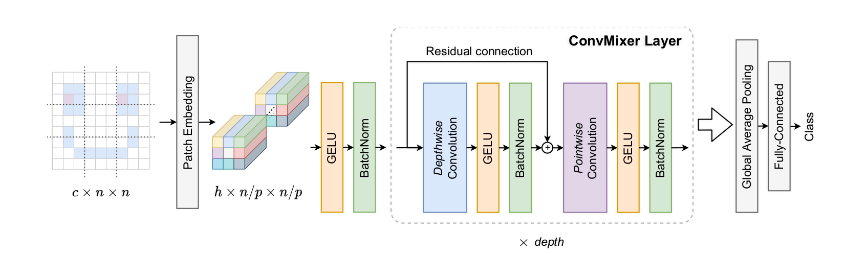
Let's decompose it block by block.

Chain

In Flux, the basic way to compose layers is Chain, the equivalent of Torch's nn.Sequential. There's nothing more to say.

Patch embedding as a convolution

The main point of the ConvMixer architecture is that it begins by splitting an image in patches of size (p, p). This is done using the convolutional layer and the stride argument. Let us take a $(p,p)$ convolution. If stride=1, the convolution is applied around every pixel in the image. If stride = 2, it is applied only on one over two pixels, etc. With stride=p, the windows on which the convolution is applied are all disjoint and adjacent, thus covering the image in $(p,p)$ patches. This is why the first layer of ConvMixer is

Conv((p, p), 3=>H, gelu; stride=p).

In Flux, the third argument of a convolution, if specified, is an activation function applied pointwise^[1]. Here, we take the Gaussian error linear unit, Gelu. Additionnaly, we transform the 3 initial RGB channels in $H$ (like hidden) dimensions. After this operation, the batch has dimension

(32/p, 32/p, H, B)

Batchnorm

In ConvMixer as in many networks, each layer is followed by a batch normalization: after being filtered, the arrays representing images in a batch are centered and reduced along each dimension. There are two learnable parameters (mean and std) for each dimension. In Flux, we simply call BatchNorm(H).

Residual networks

The next ingredient for the ConvMixer architecture is the residual connection: instead of filtering $x$ to $f(x)$ and feeding $f(x)$ to the next layer, we feed $x+f(x)$ to the next layer. In Flux, this is done with SkipConnection(layer, +) where layer is any chain of layers. Note that we are not forced to use addition + to perform the connection. We could multiply, concatenate or anything else.

We use these SkipConnections with layers composed of channel-wise convolutions: here the groups argument tells us that the convolution is applied indepedently on each channel.

SkipConnection(
    Chain(
        Conv((kernel,kernel), H=>H, gelu; pad=SamePad(), groups=H),
        BatchNorm(H)), 
    +
)

This residual layer is followed by a purely pixel-wise convolutional layer, and this whole operation is repeated depth times.

Last layers

At the end of the last convolutional layer, we have a batch of dimension $(32/p, 32/p, H, B)$ . It is time to reduce dimensions: we average over each channel with AdaptativeMeanPool((1,1)) to obtain a $(1,1,H, B)$ batch, then we apply a dense layer (which is only applied to flattened arrays, hence the flatten layer right before):

Chain(AdaptiveMeanPool((1,1)), flatten, Dense(H,N_classes))

The final implementation

using Flux

function ConvMixer(in_channels, H, k, patch, depth, N_classes)
    return Chain(
            Conv((patch, patch), in_channels=>H, gelu; stride=patch),
            BatchNorm(H),
            [
                Chain(
                    SkipConnection(
                        Chain(
                            Conv((k,k),H=>H,gelu; pad=SamePad(), groups=H), 
                            BatchNorm(H)
                        ), 
                    +),
                    Chain(Conv((1,1), H=>H, gelu), BatchNorm(H))
                ) 
                for i in 1:depth
            ]...,
            AdaptiveMeanPool((1,1)),
            flatten,
            Dense(H,N_classes)
        )
    return f
end

Let's compute the number of parameters: the patch-splitting convolution has $3 \times H\times p^2$ parameters. The BatchNorm layer has $2H$ parameters. Each of the depth layers has $H\times k^2 + 2H + H^2 + 2H$ parameters (conv, batchnorm, conv, batchnorm). The last layer is affine, hence it has $H \times N + N$ parameters. Overall we have

\mathscr{P}(k,p,H,N, \text{depth}) = 3 H p^2 + 2H + \text{depth}(Hk^2 + 4H + H^2) + NH + N

learnable parameters in this architecture^[2].

Train the mixer

The Cifar10 Dataset

Training large networks on the reference ImageNet dataset is resource-consuming. I'm sticking to the smaller dataset CIFAR10.

using MLDatasets
using Flux:onehotbatch, Dataloader

function get_CIFAR_data(batchsize; idxs = nothing)
    """
        idxs=nothing gives the full dataset.
        otherwise only the 1:idxs elements of the train set are given.
    """
    ENV["DATADEPS_ALWAYS_ACCEPT"] = "true" 

    if idxs==nothing
        xtrain, ytrain = MLDatasets.CIFAR.traindata(Float32)
        xtest, ytest = MLDatasets.CIFAR.testdata(Float32)
	else
        xtrain, ytrain = MLDatasets.CIFAR.traindata(Float32, 1:idxs)
        xtest, ytest = MLDatasets.CIFAR.testdata(Float32, 1:Int(idxs/10))
    end

    # Reshape Data to comply to Julia's convention:
    #(width, height, channels, batch_size)
    xtrain = reshape(xtrain, (32,32,3,:))
    xtest = reshape(xtest, (32,32,3,:))
    ytrain, ytest = onehotbatch(ytrain, 0:9), onehotbatch(ytest, 0:9)

    train_loader = DataLoader((xtrain, ytrain), batchsize, shuffle=true)
    test_loader = DataLoader((xtest, ytest), batchsize)

    return train_loader, test_loader
end

Flux's Dataloader splits the data in batches of the given size, possibly shuffled, and returns an iterable object whose elements are $(x,y)$ where $x$ is a batch and $y$ the corresponding labels.

Also, we shouldn't train our model on raw CIFAR10; we should augment it using classical procedures (random modifications, mixups and so on). I'll do this next time using Augmentor.jl.

GPU support

Flux uses the CUDA toolbox: the device(T) method takes any object T and puts it on device. If you have a batch of images and labels x,y drawn from your dataloader, you put it on the gpu using x = gpu(x) and back on the cpu with x = cpu(x).

Cross-entropy loss and classification accuracy

Since we deal with a classification task (there are 10 classes on CIFAR), we'll train the network using the logit cross entropy. Just for the sake of writing maths, let's recall how it works. With $C = 10$ classes, our architecture is fed an image $x_i$ , and outputs the probability $\hat{p}_{i, c}$ that this image belongs to class $c$ . The ground truth would be $p_{i,c}=0$ for all the classes $c$ except for the real class $c$ of image $x_i$ , for which $p_{i,c}=1$ . The cross-entropy (Flux.logitcrossentropy) measures this discrepancy in the following way:

L(\hat{p}_i, p_i) = - \sum_{c=1}^C \log(\hat{p}_{i,c})p_{i,c}.

We'll also keep track of the accuracy of the model: since we want to predict classes, and not only probabilities, we predict the class of an image to be the one with the highest predicted probability $\hat{p}_{i,c}$ . That's what the onecold function from Flux does. The proportion of correct predictions is the accuracy.

using Flux:onecold, logitcrossentropy

function ℓ(dataloader, model, device)
    """batch-wise loss and accuracy"""
    
    n = 0
    cross_entropy = 0.0f0
    accuracy = 0.0f0

    for (x,y) in dataloader
        x,y = x |> device, y |> device
        z = model(x)        
        cross_entropy += logitcrossentropy(z, y, agg=sum)
        accuracy += sum(onecold(z).==onecold(y))
        n += size(x)[end]
    end
    cross_entropy / n, accuracy / n
end

Training loop

Let's put everything together.

using Flux:Optimiser
using BSON:@save

function train(n_epochs=200, η=3e-4, device=gpu)

    train_loader, test_loader = get_data(128)
    patch_size = 2
    kernel_size = 7
    dim = 128
    depth = 8

    #for saving the losses and accuracy
    train_save = zeros(n_epochs, 2)
    test_save = zeros(n_epochs, 2)

    model = ConvMixer(3, kernel_size, patch_size, dim, depth, 10) |> device

    ps = params(model)
    opt = Optimiser(
            WeightDecay(1f-3), 
            ClipNorm(1.0),
            ADAM(η)
            )

    for epoch in 1:n_epochs
        for (x,y) in train_loader
            x,y = x|>device, y|>device
            gr = gradient(()->Flux.logitcrossentropy(model(x), y, agg=sum), ps)
            Flux.Optimise.update!(opt, ps, gr)
        end

        #logging
        train_loss, train_acc = ℓ(train_loader, model, device) |> cpu
        test_loss, test_acc = ℓ(test_loader, model, device) |> cpu
        train_save[epoch,:] = [train_loss, train_acc]
        test_save[epoch,:] = [test_loss, test_acc]

        if epoch%5==0
            @info "t=$epoch : Train loss = $train_loss | Test acc. = $test_acc."
        end

    end

    model = model |> cpu
    @save "save/model.bson" model 
    @save "save/losses.bson" train_save test_save
end

Some comments:

Patches are small ( $2 \times 2$ ). For small datasets like CIFAR, we don't need large patches and indeed the best results are obtained with $p=1$ . However, for experiments on larger datasets like ImageNet where pictures are $224\times 224$ , patches of sizes 7,8 or 9 perform well (all this according to the ConvMixer paper).

The optimiser includes weight decay and gradient clipping with naive parameters.
The parameters were mostly taken from the ConvMixer paper; I chose them small enough so that the training of this model roughly took one afternoon on a Tesla P100.

This network has less than 200k parameters, which is quite tiny.

Training curves

Most of the training time was spent overfitting with few improvement in the generalization error.

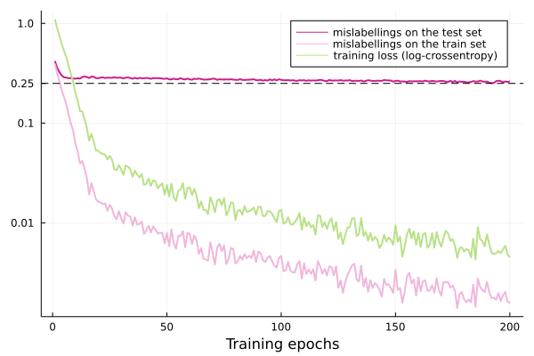
After 200 training epochs on batches of size 128, I got a labelling accuracy of 74%. That's bad, but I underoptimised nearly everything: no augmentations on the dataset, no optimiser parameter scheduler, and a pretty small network. For reference, the best performances on CIFAR are above 95%; the best ConvMixer performance seems close to 97% (with 1.3 million parameters).

I'm not a code golfer

The authors of the ConvMixer paper argue that their architecture is as powerful as ResNets or ConViT high-performance models without any hyperparameter tuning, but the conceptual complexity of the model is considerably simpler: in fact, it is simplistic enough to fit in one tweet, ie less than 280 characters when implemented with the PyTorch framework.

a single tweet

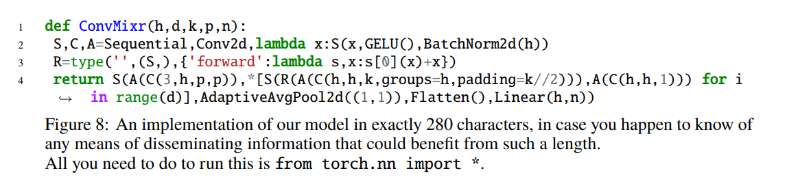
This implies a little bit of code golf cheating. In Julia, you can fit everything in a single tweet, using Flux included, in 272 characters without even needing to golf your functions names:

even better

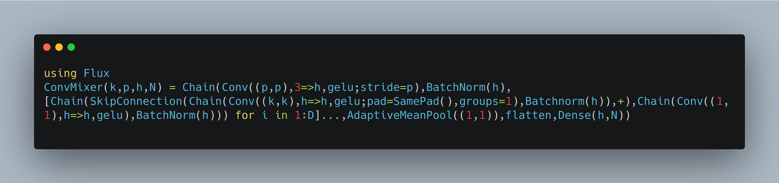
The code is here (with spaces):

ConvMixer(k,p,h,N) = Chain(Conv((p,p), 3=>h, gelu;stride=p), BatchNorm(h), [Chain(SkipConnection(Chain(Conv((k,k),h=>h,gelu;pad=SamePad(),groups=1), Batchnorm(h)),+), Chain(Conv((1,1),h=>h,gelu), BatchNorm(h))) for i in 1:D]..., AdaptiveMeanPool((1,1)), flatten, Dense(h,N))

Julia's Flux library

The main goal of this post was to give a serious try to Julia's Flux library for deep learning. In short, it works. All the needed functionalities are here: the basic building blocks of deep vison architectures (convolutions, residuals, batchnorms, nonlinearities, LSTM, RNN, etc.) - I do not know if it's the same for NLP tools of GNNs. Autodiff works well and you can easily write your own gradients using the @adjoint macro.

Using a single GPU for ML experiments is just as easy as in any other framework. GPU computing works well with CUDA.jl^[3]. I stumbled on bugs but the JuliaGPU team and @maleadt (Tim Besard) solved them at godspeed.

Last but not least, Flux benefits from the high flexibility and readability of the Julia language.

In conclusion, there are many frameworks for doing deepl learning research right now: PyTorch, TensorFlow and satellites (MXNet, Sonnet), Keras, JAX, Flux, Matlab... I'm not a fan of communities wars, but it's fair to say that overall, PyTorch won: it's more flexible, it has the largest community, it's more robust and stable. But just as Torch or TF or Keras, Flux is also excellent. It has everything we need. It's sufficiently powerful, well-documented and flexible to be used in a day-to-day basis for Machine Learning research, and most importantly, to focus on content rather than on implementation. All hail Flux!

References: the Paper Title Competition

Attention is all you need was published 4 years ago and has 33k citations.

An image is worth 16x16 words was written in 2020.

The first paper emphasizing the role of patches seems to be Do you even need attention?.

The original ConvMixer paper is Patches are all you need? - the style is quite unconventional for a conference paper 🤷.

Most of my implementation of the training loop is inspired by the excellent Flux Model Zoo, a collection of simple implementations of classical deep learning architectures.

Notes

^[1] In Torch, you would use nn.Sequential(nn.Conv2d(...), nn.GeLU()).

^[2] The Convmixer paper mentions a slightly different formula; I'm under the impression that their Batchnorm layers have $3$ learnable parameters per channel. Where am I wrong?

^[3] Unfortunately, people having a non-NVIDIA GPU will have a hard time using it, and not only with JuliaGPU. Nvidia definitely took the high ground in the GPU game for machine learning.