Diffusion models

March 2023

These notes focus on diffusion-based generative models, like the celebrated Denoising Diffusion Probabilistic Models; the material was presented as a series of lectures I gave at some working groups of mathematicians, so the style is tailored for this audience. In particular, everything is fitted into the continuous-time framework (which is not how it is done in practice).

A special attention is given to the differences between ODE sampling and SDE sampling. The analysis of the time evolution of the densities $p_t$ is done using only Fokker-Planck Equations or Transport Equations.

The problem
Original formulation: Gaussian noising process and its inversion
Methods for learning the score
Generative models: training and sampling
A variational bound for the SDE sampler
References

The problem

Let $p$ be a probability density on $\mathbb{R}^d$ . The goal of generative modelling is twofold: given samples $x^1, \dotsc, x^n$ from $p$ , we want to

learn $p$ ;
generate new samples from $p$ .

There are various methods for tackling these challenges: Energy-Based Models, Normalizing Flows and the famous Neural ODEs, vanilla Score-Matching. However, each method has its limitations. For example, EBMs are very challenging to train, NFs lack expressivity and SM fails to capture multimodal distributions. Diffusion models offer sufficient flexibility to (partially) overcome these limitations.

Stochastic interpolation

Diffusion models fall into the general framework of stochastic interpolants. The central idea is to continuously transform the density $p$ into another easy-to-sample density $\pi$ (often called the target), while also transforming the samples $x^i$ from $p$ into samples from $\pi$ ; and then, to reverse the process: that is, to generate a sample from $\pi$ , and to inverse the transformation to get a new sample from $p$ . In other words, we seek a path $(p_t: t\in [0,T])$ with $p_0=p$ and $p_T=q$ , such that generating samples $x_t \sim p_t$ is doable.

The success of diffusion models came from the realization that some stochastic processes, such as Ornstein-Uhlenbeck processes that connect $p_0$ with a distribution $p_T$ very close to pure noise $\mathscr{N}(0,I)$ , can be reversed when the score function $\nabla \log p_t$ is available at each time $t$ . Although unknown, this score can efficiently be learnt using statistical procedures called score matching.

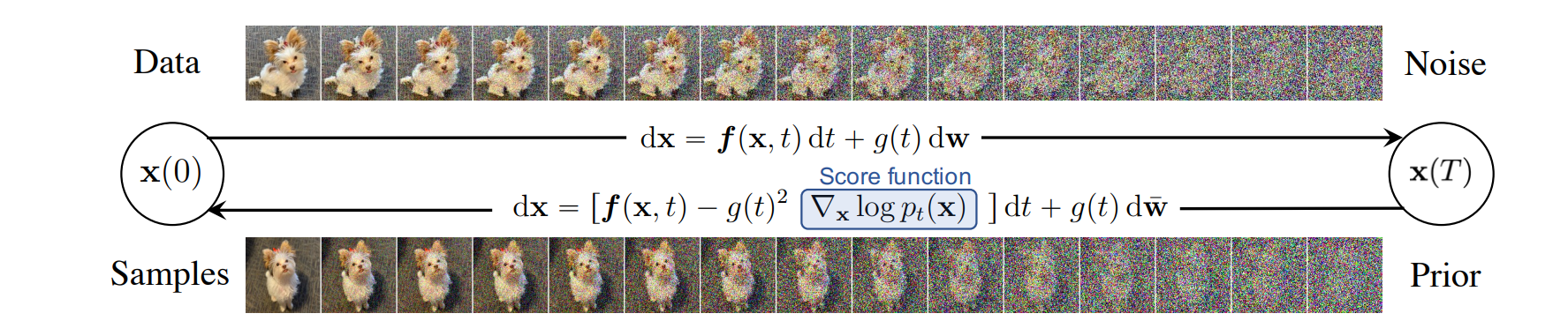
Original formulation: Gaussian noising process and its inversion

Let $(t,x)\to f_t(x)$ and $t\to \sigma_t$ be two smooth functions. Consider the stochastic differential equation

\begin{aligned}& dX_t = f_t(X_t)dt + \sqrt{2\sigma_t ^2}dB_t, \\ & X_0 \sim p\end{aligned}

where $dB_t$ denotes integration with respect to a Brownian motion. Under mild conditions on $f$ , an almost-surely continuous stochastic process satisfying this SDE exists. Let $p_t$ be the probability density of $X_t$ ; it is known that this process could easily be reversed in time. More precisely, the SDE

\begin{aligned} & dY_t = -\left( f_t(Y_t)+ 2\sigma_t^2 \nabla \log p_t(Y_t) \right)dt + \sqrt{2\sigma_t^2}dB_t \\ & Y_T \sim p_T \end{aligned}

has the same marginals as $X_t$ reversed in time: more precisely $Y_{T-t}$ has the same distribution as $X_t$ , with density noted $p_t$ . This inversion needs access to $\nabla \log p_t$ , and we'll explain later how this can be done.

For simple functions $f$ , the process (1) has an explicit representation. Here we focus on the case where $f_t(x) = -\alpha_t x$ for some function $\alpha$ , that is

dX_t = -\alpha_t X_t + \sqrt{2\sigma_t^2}dB_t.

Define

\mu_t = \int_0^t \alpha_s ds

. Then, the solution of (3) is given by the following stochastic process:

X_t = e^{-\mu_t}X_0 + \sqrt{2}\int_0^t e^{\mu_s-\mu_t} \sigma_s dB_s.

In particular, the second term reduces to a Wiener Integral; it is a centered Gaussian with variance $2\int_0^t e^{2(\mu_s-\mu_t)}\sigma_s^2 ds$ , hence

X_t \stackrel{\mathrm{law}}{=} e^{-t}X_0 + \mathscr{N}\left(0, 2\int_0^t e^{2\mu_s - 2\mu_t}\sigma_s^2 ds\right).

In the pure Orstein-Uhlenbeck case where $\sigma_t = \sigma$ and $\alpha_t = 1$ , we get $\mu_t = t$ and $X_t = e^{-t}X_0 + \mathscr{N}(0,1 - e^{-2t})$ .

Proof of (4). We set

F(x,t) = xe^{\mu_t}

and

Y_t = F(X_t, t) = X_t e^{\mu_t}

; it turns out that

Y_t

satisfies a nicer SDE. Since

\Delta_x f = 0

\partial_t f(x,t) = xe^{\mu_t}\alpha_t

and

\nabla_x f(x,t) = e^{\mu_t}

, Itô's formula says that

\begin{aligned}dY_t &= \partial_tF(t,X_t)dt + \partial_x F(t,X_t)dX_t + \frac{1}{2}\Delta_x F(t,X_t)dt \\ &= X_te^{\mu_t}\alpha_tdt + e^{\mu_t} dX_t \\ &= \sqrt{2\sigma_t^2 e^{2\mu_t}}dB_t. \end{aligned}

Consequently,

Y_t = Y_0 + \int_0^t \sqrt{2\sigma_s^2e^{2\mu_t}}dB_s

and the result holds.

A consequence of the preceding result is that when the variance

\bar{\sigma}_t^2 = 2\int_0^t e^{2\mu_s - 2\mu_t}\sigma_s^2 ds

is big compared to $e^{-\mu_t}$ , then the distribution of $X_t$ is well-approximated by $\mathscr{N}(0,\bar{\sigma}_t^2)$ . Indeed, for $\sigma_t = 1$ , we have $\bar{\sigma}_T = \sqrt{1 - e^{-2T}} \approx 1$ if $T$ is sufficiently large.

The Fokker-Planck point of view

It has recently been recognized that the Ornstein-Uhlenbeck representation of $p_t$ as in (1), as well as the stochastic process (2) that has the same marginals as $p_t$ , are not necessarily unique or special. Instead, what matters are two key features: (i) $p_t$ provides a path connecting $p$ and $p_T\sim N(0,I)$ , and (ii) its marginals are easy to sample. There are many other processes besides (1) that have $p_t$ as their marginals, and that can also be reversed. The crucial point is that $p_t$ is a solution of the Fokker-Planck equation:

\partial_t p_t(x) = \Delta (\sigma_t^2 p_t(x)) - \nabla \cdot (f_t(x)p_t(x)).

Just to settle the notations once and for all: $\nabla$ is the gradient, and for a function $\rho : \mathbb{R}^d \to \mathbb{R}^d$ , $\nabla \cdot \rho(x)$ stands for the divergence, that is $\sum_{i=1}^d \partial_{x_i} \rho(x_1, \dotsc, x_d)$ , and $\nabla \cdot \nabla = \Delta = \sum_{i=1}^d \partial^2_{x_i}$ is the Laplacian.

Importantly, equation (8) can be recast as a transport equation: with a velocity field defined as

v_t(x) = \sigma_t^2 \nabla \log p_t(x) - f_t(x),

the equation (8) is equivalent to

\partial_t p_t(x) = \nabla \cdot (v_t(x)p_t(x)).

Proof.

\nabla \cdot v_t(x)p_t(x) = \nabla\cdot \nabla (\log p_t(x))p_t(x) - \nabla\cdot f_t(x)p_t(x)= \nabla\cdot \nabla p_t(x) - \nabla\cdot f_t(x)p_t(x)

An associated ODE

Transport equations like (10) come from simple ODEs; that is, there is a deterministic process with the same marginals as (1).

Let

x(t)

be the solution of the differential equation with random initial condition

x'(t) = -v_t(x(t))\qquad \qquad x(0) =X_0.

Then the probability density of

x(t)

satisfies (10), hence it is equal to

p_t

Proof. Let

p_t

be the probability density of

x(t)

and let

\varphi

be any smooth, compactly supported test function. Then,

\mathbb{E}[\varphi(x(t))] = \int p_t(x)\varphi(x)dx

, so by derivation under the integral,

\begin{aligned}\int \partial_t p_t(x)\varphi(x)dx = \partial_t \mathbb{E}[\varphi(x(t))]&= \mathbb{E}[\nabla\varphi(x(t))x'(t)]\\ &= -\int \nabla \varphi(x)v_t(x)p_t(x)dx = \int \varphi(x) \nabla \cdot (v_t(x)p_t(x))dx \end{aligned}

where the last line uses the multidimensional integration by parts formula.

Up to now, we proved that there are two continuous random processes having the same marginal probability density at time $t$ : a smooth one provided by $x(t)$ , the solution of the ODE, and a continuous but not differentiable one, $X_t$ , provided by the solution of the SDE.

Time-reversal of Transport Equations and Fokker-Planck equations

We now have various processes $x(t), X_t$ starting at a density $p_0$ and evolving towards a density $p_T \approx \pi = \mathscr{N}(0,I)$ . Can these processes be reversed in time? The answer is yes for both of them. We'll start by reversing their associated equations. From now on, we will note $p^{\mathrm{b}}_t$ the time-reversal of $p_t$ , that is:

p^{\mathrm{b}}_t(x) = p_{T-t}(x).

The density $p^{\mathrm{b}}_t$ solves the backward Transport Equation: $\partial p^{\mathrm{b}}_t(x)= \nabla \cdot v^{\mathrm{b}}_t(x) p^{\mathrm{b}}_t(x)$ where

v^{\mathrm{b}}_t(x) = -v_t(x) = -\sigma_{T-t}^2 \nabla \log p_t(x) - \alpha_{T-t} x.

The density $p^{\mathrm{b}}_t$ also solves the backward Fokker-Planck Equation: $\partial p^{\mathrm{b}}_t(x) =\sigma_{T-t}^2 \Delta p^{\mathrm{b}}_t(x) - \nabla \cdot w_t^{\mathrm{b}}(x)p^{\mathrm{b}}_t(x)$ where

w^{\mathrm{b}}_t(x) = 2\sigma_{T-t}^2 \nabla \log p^{\mathrm{b}}_t(x) + \alpha_{T-t} x.

Proof. Noting

\dot{p}_t(x)

the time derivative of

t\mapsto p_t(x)

at time

t

, we immediately see that

\partial_t p^{\mathrm{b}}_t(x) = -\dot{p}_{T-t}(x)

and the rest is a mere verification.

Of course, these two equations are the same, but they represent the time-evolution of the density of two different random processes. As explained before, the Transport version (14) represents the time-evolution of the density of the ODE system

\begin{aligned}& y'(t) = -v^{\mathrm{b}}_t(y(t)) \\ & y(0) \sim p_T\end{aligned}

while the Fokker-Planck version (16) represents the time-evolution of the SDE system

\begin{aligned}&dY_t = w^{\mathrm{b}}_t(Y_t)dt + \sqrt{2\sigma_{T-t}^2}dB_t \\ & Y_0 \sim p_T.\end{aligned}

Both of these two processes can be sampled using a range of ODE and SDE solvers, the simplest of which being the Euler scheme and the Euler-Maruyama scheme. However, this requires access to the functions $v^{\mathrm{b}}_t$ and $w^{\mathrm{b}}_t$ , which in turn depend on the unknown score $\nabla \log p_t$ . Fortunately, $\nabla \log p_t$ can efficiently be estimated due to two factors.

First: we have samples from $p_t$ . Remember that our only information about $p$ is a collection $x^1, \dotsc, x^n$ of samples. But thanks to the representation (5), we can represent $x^i_t = e^{-\mu_t}x^i + \bar{\sigma}_t \xi^i$ with $\xi^i \sim \mathscr{N}(0,I)$ are samples from $p_t$ . They are extremely easy to access, since we only need to generate iid standard Gaussian variables $\xi^i$ .
Second: score matching. If $p$ is a probability density and $x^i$ are samples from $p$ , estimating $\nabla \log p$ (called score) has been thoroughly examined and is fairly doable, a technique known as score matching.

Methods for learning the score

The L2-distance between the scores of two probability densities is often called the Fisher divergence:

\mathrm{fisher}(\rho_1 \mid \rho_2) = \int \rho_1(x)|\nabla\log\rho_1(x) - \nabla\log\rho_2(x)|^2dx.

Since our goal is to learn $\nabla\log p_t(x)$ , it is natural to choose a parametrized family of functions $s_\theta$ and to optimize $\theta$ so that the divergence

\int p_t(x)|\nabla\log p_t(x) - s_\theta(x)|^2dx

is as small as possible. However, this optimization problem is intractable, due to the presence of the explicit form of $p_t$ inside the integral. This is where Score Matching techniques come into play.

Vanilla score matching

Let $p$ be a smooth probability density function supported over $\mathbb{R}^d$ and let $X$ be a random variable with density $p$ . The following elementary identity is due to Hyvärinen, 2005; it is the basis for score matching estimation in statistics.

Let

s : \mathbb{R}^d \to \mathbb{R}^d

be any smooth function with sufficiently fast decay at

\infty

, and

X \sim p

. Then,

\mathbb{E}[\vert \nabla \log p(X) - s(X)\vert^2] = c + \mathbb{E}\left[|s(X)|^2 + 2 \nabla \cdot s(X)\right]

where

c

is a constant not depending on

s

Proof. We start by expanding the square norm: $\begin{aligned}\int p(x)|\nabla \log p(x) - s(x)|^2 dx &= \int p(x)|\nabla \log p(x)|^2 dx + \int p(x)|s(x)|^2 dx - 2\int \nabla \log p(x)\cdot p(x)s(x) dx. \end{aligned}$ The first term does not depend on $s$ , it is our constant $c$ . For the last term, we use $\nabla \log p = \nabla p / p$ then we use the integration-by-parts formula:

2\int \nabla \log p(x)\cdot p(x)s(x) dx = 2\int \nabla p(x) \cdot s(x) dx = -2 \int p(x)( \nabla \cdot s(x))dx

and the identity is proved.

Now, (22) is particularly interesting for us. Remember that if we want to reverse (11), we do not really need to estimate $p_t$ but only $\nabla \log p_t$ . We do so by approximating it using a parametrized family of functions, say $s_\theta$ (typically, a neural network):

\theta_t \in \argmin_\theta \mathbb{E}[\vert \nabla \log p_t(X_t) - s_{\theta}(X_t)\vert^2] = \argmin_\theta \mathbb{E}[|s_{\theta}(X_t)|^2 + 2 \nabla \cdot (s_{\theta}(X_t))].

How do we empirically optimize (25)?

First, we need not solve this optimization problem for every $t$ . We could obviously discretize $[0,T]$ with $t_1, \dots, t_N$ and only solve for $\theta_{t_i}$ independently, but it is actually smarter and cheaper to approximate the whole function $(t,x) \to \nabla \log p_t(x)$ by a single neural network (a U-net, in general). That is, we use a parametrized family $s_\theta(t,x)$ . This enforces a form of time-continuity which seems natural. Now, since we want to aggregate the losses at each time, we solve the following problem:

\argmin_\theta \int_0^T w(t)\mathbb{E}[|s_{\theta}(t, X_t)|^2 + 2 \nabla \cdot (s_{\theta}(t, X_t))]dt

where $w(t)$ is a weighting function (for example, $w(t)$ can be higher for $t\approx 0$ , since we don't really care about approximating $p_T$ as precisely as $p_0$ ).

In the preceding formulation we cannot exactly compute the expectation with respect to $p_t$ , but we can approximate it with our samples $x_t^i$ . Additionnaly, we need to approximate the integral, for instance we can discretize the time steps with $t_0=0 < t_1 < \dots < t_N = T$ . Our objective function becomes

\ell(\theta) =\frac{1}{n}\sum_{t \in \{t_0, \dots, t_N\}} w(t)\sum_{i=1}^n |s_{\theta}(t, x_t^i)|^2 + 2 \nabla\cdot(s_{\theta}(t, x_t^i))

which looks computable… except it's not ideal. Suppose we perform a gradient descent on $\theta$ to find the optimal $\theta$ for time $t$ . Then at each gradient descent step, we need to evaluate $s_{\theta}$ as well as its divergence; and then compute the gradient in $\theta$ of the divergence in $x$ , in other words to compute $\nabla_\theta \nabla_x \cdot s_\theta$ . In high dimension, this can be too costly.

Denoising Score Matching

Fortunately, there is another way to perform score matching when $p_t$ is the distribution of a random variable with gaussian noise added, as in our setting. We'll present this result in a fairly abstract setting; we suppose that $p$ is a density function, and $q = p*g$ where $g$ is an other density. The following result is due to Vincent, 2010.

Denoising Score Matching Objective

Let $s:\mathbb{R}^d \to \mathbb{R}^d$ be a smooth function. Let $X$ be a random variable with density $p$ , $\varepsilon$ an independent random variable with density $g$ , and $X_\varepsilon = X + \varepsilon$ , whose density is $p_g = p * g$ . Then, $\mathbb{E}[\vert \nabla \log p_g(X_\varepsilon) - s(X_\varepsilon)\vert^2] = c + \mathbb{E}[|\nabla \log g(\varepsilon) - s(X_\varepsilon)|^2]$ where $c$ is a constant not depending on $s$ .

Proof. By the same computation as for vanilla score matching, we have

\mathbb{E}[\vert \nabla \log p_g(X_\varepsilon) - s(X_\varepsilon)\vert^2] = c + \int p_g(x)|s(x)|^2dx -2\int \nabla p_g(x)\cdot s(x)dx.

Now by definition, $p_g(x) = \int p(y)g(x-y)dy$ , hence $\nabla p_g(x) = \int p(y)\nabla g(x-y)dy$ , and the last term above is equal to $\begin{aligned} -2\int \int p(y)\nabla g(x-y)\cdot s(x)dxdy &= -2\int \int p(y)g(x-y)\nabla \log g(x-y)\cdot s(x)dydx\\ &= -2\mathbb{E}[\nabla \log g(\varepsilon)\cdot s(X + \varepsilon)]. \end{aligned}$ This last term is equal to $-2\mathbb{E}[\nabla \log g(\varepsilon)\cdot s(X_\varepsilon)]$ . But then, upon adding and subtracting the term $\mathbb{E}[|\nabla \log g(\varepsilon)|^2]$ which does not depend on $s$ , we get another constant $c'$ such that

\mathbb{E}[\vert \nabla \log p_g(X) - s(X)\vert^2] = c' + \mathbb{E}[|\nabla \log g(\varepsilon) - s(X + \varepsilon)|^2].

Now, this Denoising Score Matching loss does not involve any computation of a « double gradient » like $\nabla_\theta \nabla_x \cdot s_\theta$ .

Let us apply this to our setting. Remember that $p_t$ is the density of $e^{-\mu_t}X_0 + \varepsilon_t$ where $\varepsilon_t \sim \mathscr{N}(0,\bar{\sigma}_t^2)$ , hence in this case $g(x) = (2\pi\bar{\sigma}_t^2)^{-d/2}e^{-|x|^2 / 2\bar{\sigma}_t^2}$ and $\nabla \log g(x) = - x / \bar{\sigma}^2_t$ . The objective in (26) becomes

\argmin_\theta \int_0^T w(t)\mathbb{E}\left[\left|-\frac{\varepsilon_t}{\bar{\sigma}_t^2} - s_\theta(t, e^{-\mu_t}X_0 + \varepsilon_t) \right|^2\right]dt.

This can be further simplified. Indeed, let us slightly change the parametrization and use $r_\theta(t,x) = -\bar{\sigma}_t s_\theta(t,x)$ . Then,

\argmin_\theta \int_0^T \frac{w(t)}{\bar{\sigma}_t}\mathbb{E}\left[\left|\xi - r_\theta(t, e^{-\mu_t}X_0 + \bar{\sigma}_t \xi) \right|^2\right]dt.

Intuitively, the neural network $r_\theta$ tries to guess the scaled noise $\xi$ from the observation of $X_t$ .

Generative models: training and sampling

Let us wrap everything up in this section.

Training: learning the score

The Denoising Diffusion Score Matching loss

Let $\tau$ be a random time on $[0,T]$ with density proportional to $w(t)$ ; let $\xi$ be a standard Gaussian random variable. The DDPM theoretical objective is $\ell(\theta) = \mathbb{E}\left[\frac{1}{\bar{\sigma}_\tau}\left|\xi - r_\theta(\tau, e^{-\mu_\tau}X_0 + \bar{\sigma}_\tau \xi )\right|^2\right].$

Since we have access to samples $(x^i, \xi^i, \tau^i)$ (at the cost of generating iid samples $\xi^i$ from a standard Gaussian and $\tau^i$ uniform over $[0,T]$ ), we get the empirical version:

\hat{\ell}(\theta) = \frac{1}{n}\sum_{i=1}^n \left[\frac{1}{\bar{\sigma}_\tau}|\xi^i - r_\theta(e^{-\mu_\tau}x^i + \bar{\sigma}_\tau \xi^i)|^2\right].

Up to the constants and the choice of the drift $\alpha_t$ and variance $\sigma_t$ , this is exactly the loss function (14) from the paper DDPM, for instance.

In practice, for image generations, the go-to choice for the architecture of $r_\theta$ is a U-net, a special kind of convolutional neural networks with a downsampling phase, an upsampling phase, and skip-connections in between.

Sampling

Once the algorithm has converged to $\theta$ , we get $s_\theta(t,x)$ which is a proxy for $\nabla \log p_t(x)$ . Now, we simply plug this expression in the functions $v^{\mathrm{b}}_t$ if we want to solve the ODE (18) or $w^{\mathrm{b}}_t$ if we want to solve the SDE (19).

The ODE sampler solves

y'(t) = -\hat{v}^{\mathrm{b}}_t(y(t))

started at

y(0) \sim \mathscr{N}(0,I)

, where

\hat{v}^{\mathrm{b}}_t(x) = -\sigma_{T-t}^2 s_\theta(T-t,x) - \alpha_{T-t} x

The SDE sampler solves

dY_t = \hat{w}^{\mathrm{b}}_t(Y_t)dt + \sqrt{2\sigma_t^2}dB_t

started at

Y_0 \sim \mathscr{N}(0,I)

, where

\hat{w}^{\mathrm{b}}_t(x) = 2\sigma_{T-t}^2 s_\theta(T-t,x) + \alpha_{T-t} x

We must stress a subtle fact. Equations (8) and (10), or their backward counterparts, are exactly the same equation accounting for $p_t$ . But since now we replaced $\nabla \log p_t$ by its approximation $s_\theta$ , this is no longer the case for our two samplers: their probability densities are not the same. In fact, let us note $q^{\mathrm{ode}}_t,q^{\mathrm{sde}}_t$ the densities of $y(t)$ and $Y_{t}$ ; the first one solves a Transport Equation, the second one a Fokker-Planck equation, and these two equations are different.

Backward Equations for the samplers

\partial_t q^{\mathrm{ode}}_t(x) = \nabla \cdot \hat{v}^{\mathrm{b}}_t(x)q^{\mathrm{ode}}_t(x)\qquad \qquad q_0^{\mathrm{ode}} = \pi

\partial_t q^{\mathrm{sde}}_t(x) = \nabla \cdot [\sigma_{T-t}^2\nabla \log q^{\mathrm{sde}}_t(x) - \hat{w}^{\mathrm{b}}_t(x)]q^{\mathrm{sde}}_t(x) \qquad \qquad q_0^{\mathrm{sde}} = \pi

Importantly, the velocity $\sigma_{T-t}^2\nabla \log q^{\mathrm{sde}}_t(x) - \hat{w}^{\mathrm{b}}_t(x)$ is in general not equal to the velocity $\hat{v}^{\mathrm{b}}_t(x)$ . They would be equal only in the case $s_\theta(t,x) = \nabla \log p_t(x)$ .

Proof. Since

y(t)

is an ODE, it directly satisfies the transport equation with velocity

\hat{v}^{\mathrm{b}}_t

. Since

Y_t

is an SDE, it satisfies the Fokker-Planck equation associated with the drift

\hat{w}^{\mathrm{b}}_t

, which in turn can be transformed in the transport equation shown above.

Special choices for $\alpha_t$ and $\sigma_t$

Considerable work has been done (mostly experimentally) to find good functions $\alpha_t,\beta_t$ . Some choices seem to stand out.

the Variance Exploding path takes $\alpha_t = 0$ (that is, no drift) and $\sigma_t$ a continuous, increasing function over $[0,1)$ , such that $\sigma_0 = 0$ and $\sigma_1 = +\infty$ ; typically, $\sigma_t = (1-t)^{-1}$ .
the Variance-Preserving path takes $\sigma_t = \sqrt{\alpha_t}$ .
the pure Ornstein-Uhlenbeck path takes $\alpha_t = \sigma_t = 1$ , it is a special case of the previous one, mostly suitable for theoretical purposes.

A variational bound for the SDE sampler

Let $s : [0,T]\times \mathbb{R}^d \to \mathbb{R}^d$ be a smooth function, meant as a proxy for $\nabla \log p_t$ . Our goal is to quantify the difference between the sampled densities $q^{\mathrm{ode}}_t, q^{\mathrm{sde}}_t$ and $p^{\mathrm{b}}_t=p_{T-t}$ . It turns out that controlling the Fisher divergence $\mathbb{E}[|\nabla \log p_t(X) - s(t,X)|^2]$ results in a bound for $\mathrm{kl}(p \mid q_T^{\mathrm{sde}})$ , but not for $\mathrm{kl}(p \mid q_T^{\mathrm{ode}})$ .

Small recap on notations

The true density is $p^{\mathrm{b}}_t = p_{T-t}$ , it satisfies the backward equation (14):

\partial_t p^{\mathrm{b}}_t(x) = \nabla \cdot v^{\mathrm{b}}_t(x)p^{\mathrm{b}}_t(x)\qquad \qquad v^{\mathrm{b}}_t(x) = -\sigma_{T-t}^2\nabla \log p^{\mathrm{b}}_t(x) - \alpha_{T-t}x.

The density of the generative process is $q^{\mathrm{sde}}_t$ , but we'll simply note $q_t$ . It satisfies the backward equation (37)

\partial_t q_t(x) = \nabla\cdot u_t(x)q_t(x)

where

u_t(x) = \sigma_{T-t}^2\nabla \log q_t(x) - 2\sigma_{T-t}^2s(t,x) - \alpha_{T-t}x.

The original distribution we want to sample is $p = p_0 = p^{\mathrm{b}}_T$ , and the output distribution of our SDE sampler is $q^{\mathrm{sde}}_T = q_T$ . Finally, the distribution $p_T = p_0^{\mathrm{b}}$ is approximated with $\pi$ (in practice, $\mathscr{N}(0,I)$ ).

The KL divergence between densities $\rho_1, \rho_2$ is

\mathrm{kl}(\rho_1 \mid \rho_2) = \int \rho_2(x)\log(\rho_2(x)/ \rho_1(x))dx.

A variational lower-bound

This theorem restricts to the case where the weights $w(t)$ are constant, and for simplicity, they are set to 1.

Variational lower-bound for score-based diffusion models with SDE sampler

\mathrm{kl}(p \mid q_T^{\mathrm{sde}}) \leqslant \mathrm{kl}(p_T \mid \pi) +\int_0^T \sigma^2_{t} \mathbb{E}[ |\nabla \log p_t(X_t) - s(t,X_t)\vert^2 ] dt.

The original proof can be found in this paper and uses the Girsanov theorem applied to the SDE representations (1)-(2) of the forward/backward process. This is utterly complicated and is too dependent on the SDE representation. The proof presented below only needs the Fokker-Planck equation and is done directly at the level of probability densities.

The following lemma is interesting on its own since it gives an exact expression for the KL divergence between transport equations.

\frac{d}{dt}\mathrm{kl}(p^{\mathrm{b}}_t \mid q_t) = \sigma^2_{T-t} \int p^{\mathrm{b}}_t(x) \nabla \log\left(\frac{p^{\mathrm{b}}_t(x)}{q_t(x)}\right) \cdot \left(u_t(x)- v^{\mathrm{b}}_t(x) \right)dx

In our case with the specific shape assumed by $u_t, v^{\mathrm{b}}_t$ , we get the following bound:

\begin{aligned}\frac{d}{dt}\mathrm{kl}(p_t \mid q_t) \leqslant \sigma^2_{T-t}\int p^{\mathrm{b}}_t(x) |s(t,x) - \nabla \log p^{\mathrm{b}}_t(x) |^2 dx \end{aligned}

The proofs of (42)-(43)-(44) are only based on elementary manipulations of time-evolution equations.

Proof of (43).

A small differentiation shows that $\frac{d}{dt}\mathrm{kl}(p^{\mathrm{b}}_t \mid q_t)$ is equal to

\int \nabla \cdot (v^{\mathrm{b}}_t(x)p^{\mathrm{b}}_t(x))\log(p^{\mathrm{b}}_t(x)/q_t(x))dx + \int p^{\mathrm{b}}_t(x)\frac{\nabla \cdot (v^{\mathrm{b}}_t(x)p^{\mathrm{b}}_t(x))}{p^{\mathrm{b}}_t(x)}dx - \int p^{\mathrm{b}}_t(x)\frac{\nabla \cdot (u_t(x)q_t(x))}{q_t(x)} dx.

By an integration by parts, the first term is also equal to $-\int p^{\mathrm{b}}_t(x)v^{\mathrm{b}}_t(x)\cdot \nabla \log(p^{\mathrm{b}}_t(x)/q_t(x))dx$ . For the second term, it is clearly zero. Finally, for the last one, $\begin{aligned} - \int p^{\mathrm{b}}_t(x)\frac{\nabla \cdot (u_t(x)q_t(x))}{q_t(x)} dx &= \int \nabla (p^{\mathrm{b}}_t(x)/q_t(x)) \cdot u_t(x)q_t(x)dx \\ &= \int \nabla \log(p^{\mathrm{b}}_t(x)/q_t(x))\cdot u_t(x)p^{\mathrm{b}}_t(x)dx. \end{aligned}$

Proof of (44). We recall that

u_t(x) = \sigma^2_{T-t}\nabla \log q_t(x) - 2\sigma^2_{T-t}s(t,x) - \alpha_{T-t}x

and

v^{\mathrm{b}}_t(x) = -\sigma^2_{T-t}\nabla \log p^{\mathrm{b}}_t(x) - \alpha_{T-t}x,

so that $\begin{aligned} u_t - v^{\mathrm{b}}_t &= \sigma^2_{T-t}\nabla \log q_t - 2\sigma^2_{T-t}s + \sigma^2_{T-t}\nabla \log p^{\mathrm{b}}_t\\ &= \sigma^2_{T-t} \left( \nabla \log q_t - \nabla \log p^{\mathrm{b}}_t + 2 (\nabla \log p^{\mathrm{b}}_t - s) \right).\end{aligned}$ We momentarily note $a = \nabla \log p^{\mathrm{b}}_t(x)$ and $b = \nabla \log q_t(x)$ and $s=s(t,x)$ . Then, (43) shows that $\begin{aligned} \frac{d}{dt}\mathrm{kl}(p^{\mathrm{b}}_t \mid q_t) &= \sigma^2_{T-t}\int p^{\mathrm{b}}_t(x)(a - b)\cdot ((b-a) + 2(s - a))dx\\ &= - \sigma^2_{T-t}\int p_t(x)|a-b|^2 dx + 2 \sigma^2_{T-t}\int p_t(x)(a-b)\cdot (s-a)dx. \end{aligned}$ We now use the classical inequality $2(x\cdot y) \leqslant |x|^2 + |y|^2$ ; we get

\frac{d}{dt}\mathrm{kl}(p^{\mathrm{b}}_t \mid q_t) \leqslant \sigma^2_{T-t} \int p^{\mathrm{b}}_t(x)|s(t,x) - \nabla\log p^{\mathrm{b}}_t(x)|^2dx.

Proof of (42).

Now, we simply write $\begin{aligned} \mathrm{kl}(p^{\mathrm{b}}_T \mid q^{\mathrm{sde}}_T) - \mathrm{kl}(p^{\mathrm{b}}_0 \mid q_0^{\mathrm{sde}}) &= \int_0^T \frac{d}{dt}\mathrm{kl}(p^{\mathrm{b}}_t \mid q_t) dt \end{aligned}$ and plug (44) inside the RHS. Here $q_0 = \pi$ and $p^{\mathrm{b}}_T= p$ , hence the result.

What about the ODE ?

It turns out that the ODE solver, whose density is $q^{\mathrm{ode}}_t$ , does not have such a nice upper bound. In fact, since $q^{\mathrm{ode}}_t$ solves a Transport Equation, we can still use (43) but with $u_t$ replaced with $\hat{v}^{\mathrm{b}}_t$ , and integrate in $t$ just as in (52). We have

\begin{aligned}\hat{v}^{\mathrm{b}}_t(x) - v^{\mathrm{b}}_t(x) &= \nabla \log p^{\mathrm{b}}_t(x)-s(t,x) \\ &= \nabla \log p^{\mathrm{b}}_t(x) - \nabla\log q_t(x) + \nabla\log q_t(x) - s(t,x). \end{aligned}

Using the Cauchy-Schwarz inequality, we could obtain the following upper bound.

\begin{aligned} \mathrm{kl}(p \mid q_T^{\mathrm{ode}}) - \mathrm{kl}(p_T \mid \pi) &\leqslant \int_0^T \int p_t(x)\left|\nabla\log p_t(x) - \nabla\log q_t(x)\right|^2 + p_t(x)\left|\nabla \log q_t(x) - s(t,x)\right|^2 dx dt\\ &\leqslant \int_0^T \mathbb{E}\left[|\nabla\log p_t(X_t) - \nabla\log q_t(X_t)|^2 + |\nabla\log q_t(X_t) - s(t,X_t)|^2\right]dt. \end{aligned}

There is a significant difference between the score matching objective function and the SDE version. Minimizing the former does not minimize the upper bound, whereas the latter does. This disparity is due to the Fisher divergence, which does not provide control over the KL divergence between the solutions of two transport equations. However, it does regulate the KL divergence between the solutions of the associated Fokker-Planck equations, thanks to the presence of a diffusive term. This could be one of the reasons for the lower performance of ODE solvers that was observed by early experimenters in the field. However, more recent works (see the references just below) seemed to challenge this idea. With different dynamics than the Ornstein-Uhlenbeck one, deterministic sampling techniques like ODEs seem now to outperform the stochastic one. A complete understanding of these phenomena is not available yet; the outstanding paper on stochastic interpolants proposes a remarkable framework towards this task (and inspired most of the analysis in this note).