The double descent phenomenon
November 2021Machine learning, the summary
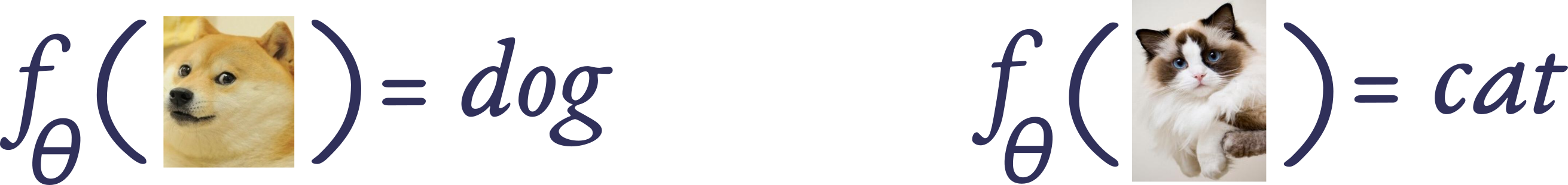
Neural networks are functions built by combining linear and non-linear functions; they depend on a certain number of parameters . Learning consists in finding the best set of parameters for performing a precise task - for instance translating text or telling if it's a cat or a dog in the photo.
In supervised learning, this is done by learning this task, say , on a set of examples where is an input and the output related to the input. We try to find such that for all the examples at our dispositions: this is called interpolation. Once this is done, we hope that did not only learn the examples, but that when confronted to unseen examples , the predicted output will be very close to the real output . This is called generalization.
The tradeoff between learning and understanding
Old school learning: overfitting vs generalizing
There's a tradeoff between interpolation and generalization. If we want a function to perfectly interpolate the data, that is, , then there's a risk of choosing too complicated given the data, and unrealistic.
For instance, suppose we want to interpolate the green points in the figure below - these points are 0 plus a very small noise. There is a big difference between:
the best linear approximation (blue curve, here and )
the best degree-6-polynomial approximation (orange line, here and ):
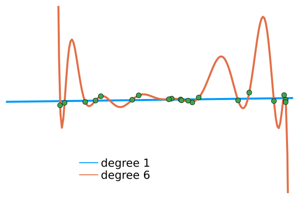 Intuitively, the second approximation (degree 6 polynomials) is more complex than the first one, so it fits better the data, but it probably not captured the phenomenon which created the green points. If I draw another green point (ie, a random Gaussian number with a small variance), there's a good chance that the orange line will be completely off, but not the blue one.
This phenomenon has been known for long; in classical statistics, it's called the bias-variance tradeoff. In short, when the complexity of increases, we should first have a better fitting of the training data and a better generalization (the model is better), but at some point, adding complexity to will fit the data too much and will not generalize well to unseen examples (the model is worse). This is called overfitting.
Deep learning overfits and generalizes
The unsettling thing with deep learning is that this is not the end of the story, and there is something beyond overfitting: with modern neural network architectures, the generalization error first decreases with the number of parameters, then increases just as explained above, and then, when the number of parameters becomes huge (heavily overparametrized regime), the generalization error decreases again. In the end, networks with a number of parameters well beyond the number of examples perform extremely well, that's one of the main successes of deep learning.
This double descent phenomenon in deep learning was discovered in 2018, see the original paper by Belkin et al., and was extensively explored after. An overview of all the double descent curves found when training huge networks (such as ResNets) on image processing tasks can be seen in OpenAI's paper on the topic. For instance, here is their double descent curve when training ResNet18 (the number of parameters is ) on CIFAR10:  The green curve is the interpolation error: unsurprisingly, it monotonously decreases, since the network better fits the images in the train set, and quickly reaches zero, a point at which the training data are perfectly interpolated. The blue curve is the test error, and increases again in the overfitting phase, but then decreases again even though the training error already vanished.
Why? The random features model
In short, there is no theoretical explanation for the double descent phenomenon, but there are some toy models in which the key features of double descent appear. Belkin, Hsu and Xu introduced some linear models and Fourier models, but the absence of non-linearities made the analogy with what happens in deep learning dubious. More recently, the paper by Mei and Montanari (2019) rigorously showed the double descent phenomenon for the Random Features model, and this is what I'll be presenting now.
The task
The underlying task to be learned is , where the inputs are -dimensional ( for the rest of the note) and is a unit vector in chosen beforehand and fixed forever. The noise can be chosen Gaussian with a small standard error of .
For the set of examples, we will draw some random inputs on and we will have at our disposition the corresponding outputs . The number of training examples will be fixed to .
d = 100 ; n = 300 ; ϵ = .001
β = randn(1, d)
x = randn(d,n)
y = sum(β.*x, dims=1) + 0.01 .* randn(1, n)
The shape of interpolating function
We try to learn by approximationg with functions that look like this:
where is a nonlinearity (typically, a ReLu), the are elements of called features and the are real numbers.
In theory, we should learn the best possible and , but this is mathematically too hard to analyze, so we simplify the problem: we will only learn ; the will be chosen at random and fixed forever. This is called the random feature regression.
In order to see how regularization affects the problem, we also use a ridge penalty of strength , so that our learning process consists in minimizing the function
This problem has a unique minimizer given by
where .
Now, if we choose a number of parameters , we immediately have our optimal parameters for learning the task given above through the examples x,y. Once we have this solution, we can compare with the real model . What we want to compute is nothing else than the error done on a new realization of , that is,
where is drawn at random. What Mei and Montanari did is to compute this quantity –- or rather, its limit in the large-dimensional regime. The formula is really involved, but we can estimate the error by drawing many realizations of and averaging over (say) 10000 realizations. We also try several ridge parameters .
function compute_test_error(x, y, p, λ)

    RF = randn(p,d) #random feature matrix with p features

    Z = relu.(RF*x)
    θ_opt = y * transpose(Z) * inv( (Z*transpose(Z)) + (λ*n/d).*I) ./ n

    x_test = randn(d, 10000)
    y_test = sum(β.*x_test, dims=1) + 0.01 .* randn(1, 10000)
    y_pred = sum(θ_opt.*relu(RF.*x), dims=1)

    return sum(y_test - y_pred)^2 ./ 10000

end
And now, let's plot this test error for a wide range of and various ridge parameters . The y-axis is the test error in (4), averaged over 10 runs, as a function of the relative number of parameters per training samples ; I took so the max number of parameters is approximately . The interpolation threshold happens at , that is, when the number of features is equal to the number of training samples.

Note that the double descent becomes milder when the ridge parameter grows. In fact, ridge penalizations as in (2) were precisely designed to avoid overfitting, by penalizing the parameters which are too high. On the other side, when , the ridge regression approaches the classical linear regression, and it can be shown that the test error at the interpolation threshold goes to - a simple computation done in Belkin's original paper.
The interesting aspect of this experiment is not only that we see the double descent, but that it's actually provable - there is a function of the number of parameters such that the error with parameters is asymptotically close to when goes to (in a certain regime, though, where is proportional to ).
A wild guess
The task we tried to learn is the simplest one: is linear. A simple linear regression would have done the job very well: in fact, adding the non-linearities only complicated the learning of .
The double descent curve might come from the fact that the complexity of our models is well too high for the task we try to learn. And if so, then maybe classical image recognition tasks like cats & dogs or MNIST are indeed way easier than we think, and highly complex ResNets architectures are way too complicated for them - but finding the exact, simple architecture suited for these tasks might also be out of reach for the moment.
References
The first motivated studies of the double descent phenomenon are due to Belkin and his team, notably in this paper and this one where they empirically show double descents in a variety of contexts, and give a theoretical tractable model where a similar phenomenon happens (linear random regression and random Fourier features).
From the experimental point of view, the reference seems to be the Deep double descent paper by an OpenAI team - some figures therein were probably among the most expensive experimentns ever done in machine learning, both in $$$ and in CO2.
A physicist approach on the double descent: double trouble in double descent and the triple descent phenomenon.
The random features model was rigorously studied in Mei and Montanari's paper.