🐘 The Elephant Random Walk
May 2023, refreshed in early 2026In the Simple Random Walk (ERW), a walker moves in random directions; all of her steps are independent. The variance of the displacement of a random walker after steps typically grows linearly with : for example in the 1d symmetric random walk defined by
with , one has . This behaviour is called diffusive, because it is a discrete analog of heat dissipation.
The introduction of long-term memory in Random Walks breaks this diffusive behaviour. In the Simple Random Walk, the walker takes a random step independently of its former moves, oblivious of her past; but instead, she could remember one of her previous steps and reproduce it, just like Elephants whose memory is said to be surprisingly vast. The Elephant Randow Walk (ERW) has been thoroughly studied since its introduction in the paper Elephants can always remember by Schütz and Trimper, both for its mathematical tractability and rich behaviour.
Here is a description of the Elephant Randow Walk (ERW) with memory parameter .
The Elephant starts at 0 and takes a first step with initial probability or with probability ; the influence of is quite subtle, we’ll explain it later.
Then, at time , the Elephant randomly remembers one of the steps she took in the past; each of the former steps has the same chance to be remembered. Then, with probability , she reproduces this step; otherwise she goes the opposite way.
Formally, we set . The first step is with some probability .
At step , let be the « remembered past step » and let be whether the elephant goes in the same or opposite direction, that is and .
The -th step is , with the last step .
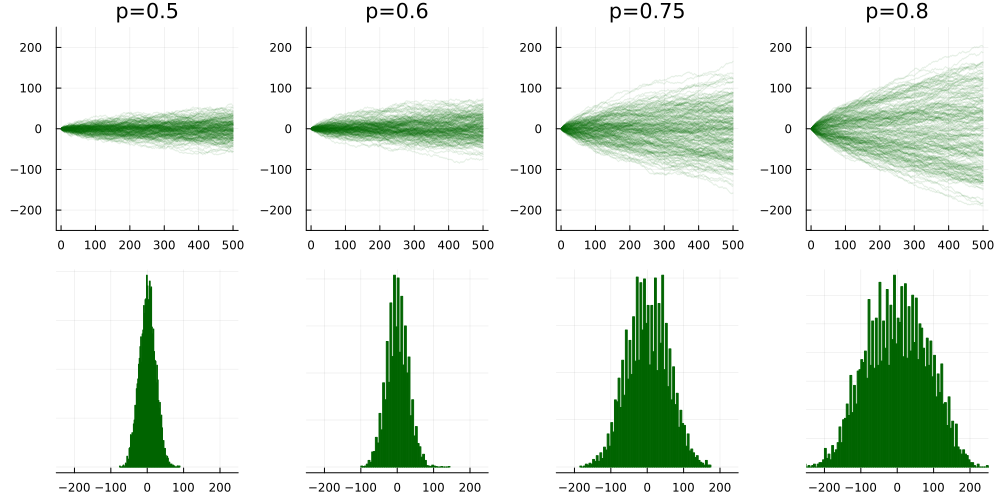
When the memory parameter is close to (full memory), the Elephant tends to reproduce always the same steps, thus going way further than the Simple Randow Walker corresponding to , and the histogram of its final position is less concentrated.
The goal of this note is to explain the appearance of a sudden and surprising transition, happening at the critical value : the ERW is still diffusive for , and becomes super-diffusive if . It all boils down to computing the variance.
Computing the variance
When the initial step has a probability to jump left or right, the whole ERW is symmetric, hence centered. Its variance solves the following recursion.
Proof. We note the sigma-algebra generated by the jumps up to time . We have
Conditionnally on , the last jump is distributed as a Rademacher random variable with a certain parameter . Let denote the number of +1 jumps before ; then . Since , we obtain
The expectation of a Rademacher random variable with parameter is , hence
which gives (2) when plugged back in the first expression.
The proof is postponed to later. This expression might not be very informative at first sight, but its large- asymptotics are easily understood and unveil a qualitative change in the behaviour of the ERW at the critical value . By symmetry we restrict to .
Diffusive case: if ,
Critical case: if ,
Super-diffusive case: if ,
Proof. Let us note the integral in (6). Its behaviour depends on wheter is positive or negative. We'll make use of Stirling's formula, , which ensures that
Now,
If then ;
If then ;
If then
Here is a log-plot of the empirical variance of 100 runs of Elephant Randow Walks with various memory parameters ranging between and . 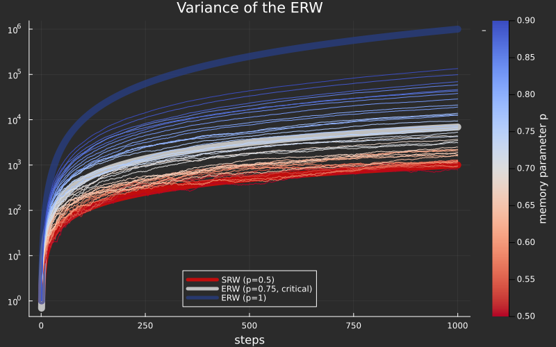 The white line marks the transition at , between a diffusive behaviour and a super-diffusive behaviour. The red line represents the Simple Random Walk with a variance of .
Proof of (6): exact computation of the variance
Recursions like (2) are easy to solve. Let us note and so that . Define
and –- we chose so that . Then, (2) becomes
By a telescoping sum and using ,
Now we see that
hence the exact formula
Now since , we get
This expression can be further simplified using the formula, valid as soon as (this is the case when ).
The limiting distribution
The variance computation above is enough to show the existence of a transition in the behaviour of the ERW. However, it does not tell the whole story. Indeed, scaling limits for the ERW are now quite well understood. In the superdiffusive case, which is the most interesting one, the scaling limit was proved essentially in Baur and Bertoin’s paper (see the references after): they proved the existence of a random variable , depending on , the probability of the very first step going up, and such that with probability 100%, we have
This random variable is, still today, quite mysterious! In a very good paper by Guérin, Laulin, Raschel and Simon, I found some of its properties:
It’s not symmetric, which is not really a surprise, but it is supported on , and it is log-concave for some range in .
It is unimodal, which rougly means that it’s increasing, then decreasing past a certain point.
Obviously, by conditionning on the firs step of the ERW, we have the identity in distribution where .
It has a density on .
And, which was (at least to me) a surprise, it is sub-gaussian, with tails that typically behave like , for various explicit constants , which also implies that they have all their moments finite, and we can even find a recursion for them. I say that it is a surprise, because in the beginning I had the intuition that was heavy-tailed. That is wrong: all the potentially heavy-tailed behaviour was suck into the nondiffusive scaling .
Conclusion and references
Many aspects of the ERW are now well understood. Its introduction in the papers Elephants can always remember and Anomalous dynamics… was mostly motivated by the physics of non-Markovian diffusions; they even formulated the continuous-time version with a non-diffusive Fokker-Planck equation. The effect of the type of memory on diffusive properties was studied in this paper.
Mathematically, the functional limit for the ERW was proved in a very elegant way in this paper – it appears that the ERW converges towards a continuous Gaussian process with a particular covariance kernel. The use of martingale theory turned out to be very powerful and allows for an efficient identification of the scaling limits of the ERW, see Bercu's paper. Multi-dimensional versions were studied in this paper.
The limiting distribution of is studied at lengths in this paper by Guérin et al.