🏋🏼 Heavy-tails II: is it really heavy?
December 2023In the preceding note on heavy tails, we defined heavy-tailed distributions as distributions for which the excess function decays polynomially fast towards zero, and not exponentially fast (as for Gaussians for example). Formally, we asked
where is some unspecified function with slow variation (ie, at infinity it is almost a constant, like ) and is called the heavy-tail index.
This raises two questions, which are statistical in nature. Suppose you are given samples from a same distribution.
How do check if their common distribution is heavy-tailed?
How do you estimate its tail index ?
In this post, we'll focus on the second question, which in practice often solves the first one. For illustration purposes, I generated three datasets whose histograms (in log-log scales) are the following ones:
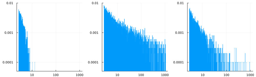
The first one does not really look heavy-tailed. The two others sure look like heavy tails. But what could possibly be their index?
Naive estimators: histograms and rank plots
Histogram
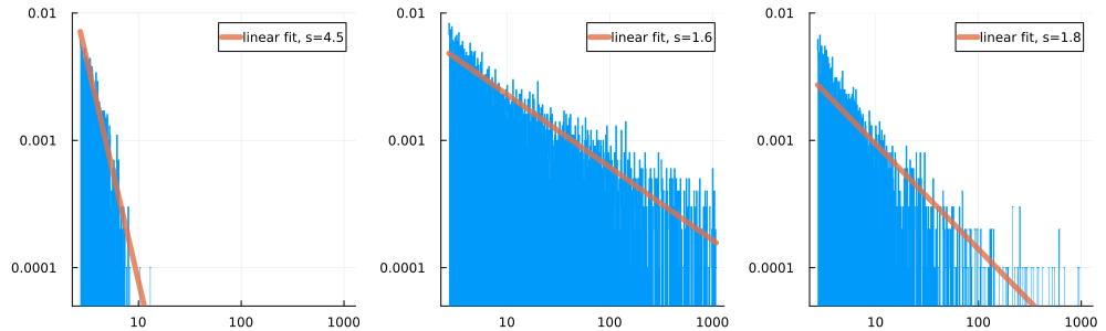
In a histogram, we count the number of observations on small bins, say . The proportion of observations in any bin should be . The tails of the histogram should thus decay like . We can also use this idea to estimate : suppose that is the height of the bin . Then we should have and so . With a linear regression of on we get an estimate for .
Rank plot
There is a better way: instead of drawing histograms, one might draw "rank plots": for every , plot the number of observations larger than . These plots are less sensitive to noise in the observations.
![]()
Again, we can use this idea to estimate the tail-index . Indeed, if is the proportion of observations greater than , then we should have , or . A linear regression would give another estimate, directly for .
![]() That's better, but still not very convincing.
That's better, but still not very convincing.
Estimating the tail index in a Pareto model
Computing the Maximum-likelihood estimator
If we suspect that the were generated from a specific parametric family of densities (Pareto, Weibull, etc.), we can try to estimate the tail-index using methods from classical parametric statistics, like Maximum Likelihood. Suppose we know that the come from a Pareto distribution, whose density is over . The likelihood of the observations is then
which is maximized when . Consequently, the MLE estimator for is:
If the were truly generated by a Pareto model, this estimator has good properties: it is consistent and asymptotically Gaussian, indeed is approximately when is large. This opens the door to statistical significance tests.
For the three datasets showed earlier, the MLE estimators are:
| 1.7 | 0.43 | 1.1 |Up to now, with three different estimators, we had very different estimates for …
Censoring
But what if my data are not Pareto-distributed? A possible approach goes as follows. Suppose that the follow some heavy-tailed distribution with density and that for some constant . Then it means that, for large , the density is almost the same as a Pareto. Hence, we could simply forget about the which are too small and only keep the large ones above some threshold (after all, they are the ones responsible for the tail behaviour), then apply the MLE estimator. This is called censorship; typically, if is the number of observations above the chosen threshold, then
This estimator is bad. Indeed,
it is biased and/or not consistent for many models[1].
It is extremely sensitive to the choice of the threshold .
To avoid these pitfalls, the idea is to play with various levels of censorship ; that is, to choose a threshold which grows larger with . This leads to the Hill estimator.
Hill's estimator
What would be the best choice for in (4)? First, we note that undergoes discontinuous changes when becomes equal to one of the , since in this case one term is added to the sum and the number of indices such that is incremented by 1. It is thus natural to replace with the largest samples, say where are the ordered samples:
Here, is the number of larger than , so (5) fits the definition of the censored estimator (4) with . The crucial difference with (4) is that the threshold is now random.
We still have to explain how to choose . It turns out that many choices are possible, and they depend on , as stated by the following essential theorem.
Proof in the case of Pareto random variables. If the have the Pareto density , then it is easy to check that are Exponential random variables with rate . The distribution of the ordered tuple is thus the distribution of . This distribution has a very nice representation due to the exponential density. Indeed, for any test function ,
in other words has the same distribution as . As a consequence,
Proof in the general case. It is rougly the same idea, but with more technicalities coming from the properties of slowly varying functions. To give the sketch, if is the cdf of the law of the , then we can write where the are uniform on . It turns out that if satisfies (??), then its inverse can be written as – this is a difficult result due to Karamata. Then, can be represented as
The first term is precisely an random variable, hence the analysis of the Pareto case holds. Then, we must show that the second term, when summed over , does not contribute. This is again a consequence of slow variation.
Typically, could be or or even . That leaves many possible choices. In practice, instead of picking one such , statisticians prefer plotting for all the possible and observe the general shape of the plot of , which is called Hill's plot. Of course, Hill's theorem above says that most of the information on is contained in a small region at the beginning of the plot, a region where is small with respect to (ie ), but not too small (ie ). It often happens that the Hill plot is almost constant on this small region, which can be seen for example in the second plot.
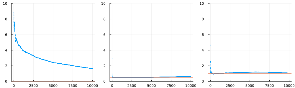
There's a whole science for reading Hill plots.
It turns out that the three datasets I created for this post are as follows:
the first one is an exponential distribution with parameter . It has a light tail.
the second one is a Pareto distribution with index .
the third one is (the absolute of) a Cauchy distribution, therefore its index is .
References
Hill's estimator. Hill's PhD-grandfather was Wald.
The manual Fundamentals of heavy tails is very clear on this topic.
[1] It is easy to see that if the come from a mixture of two Pareto distributions with different parameters , then the censored MLE estimator will not converge towards the true tail index wich is .