The Kelly criterion, crypto exchange drama, and your own utility function

November 2022

Better is bigger

There's been a lot of fuss recently on the FTX collapse and the spiritual views of his charismatic (?) 30-year old founder Sam Bankman-Fried (SBF). In a twitter thread, SBF mentioned his investment strategy and his own version of a plan due to the mathematician John L. Kelly. Further discussions (especially this one by Matt Hollerbach) pointed that he missed Kelly's point. Sam's misunderstanding prompted him to go for super-high leverage, which resulted in very risky positions – and in fine, a bankrupcy.

Fixed-fraction strategies

Here's the setting: you are in a situation where, for $n$ epochs, you can gamble money. At each epoch you can win with probability $p$, and if you win you get $w$ times your bet. If you lose (with proba $q=1-p$) you lose $\ell$ times your bet. Therefore, if you bet $1€$, your expected gain is

$$e = p w -q\ell.$$

And if you bet $R$, your expected gain is $Re$.

John L. Kelly, in his 1956 paper, asked and solved the following question:

His solution is this famous Kelly criterion, otherwise dubbed Fortune's formula in the bestseller of the same name by W. Poundstone, and became part of the history of the legendary team around Shannon who more or less disrupted some casinos in Las Vegas's Casino's in the 60s. Here's a short presentation.

Small formalization

We set $X_t = 0$ or $1$ according to the outcome of the $t$-th bet and we note $S_t = X_1+\dotsb+X_t$ the total number of wins before $t$. Starting with an initial wealth of $1$ (million), at each epoch we bet a constant fraction $0 \leqslant f \leqslant 1$ of our total wealth. Then, our wealth at epoch $t$ is

$$R_t = (1+fw)^{S_t}(1-f\ell)^{t-S_t} = (1-f\ell)^t \gamma^{S_n}$$

where $\gamma = (1+fw)/(1-f\ell)$.

Going full degenerate

A no-brain strategy^[1] to maximize the final gain $R_n$ is to compute $\mathbb{E}[R_n]$ and then optimise in $f$. Using independence,

$$\mathbb{E}[R_t] =(\mathbb{E}[\gamma^{X_1}])^t = (1-f\ell)^t (p\gamma + 1-p)^t = (1+f(pw - lq))^t = (1+fe)^t$$

and now we seek $f_\mathrm{degen}$ which maximizes this function. Clearly $(1 + fe)^n$ is increasing or decreasing according to $e>0$ or $e<0$; indeed, let us suppose that $e>0$ (the expected gain is positive), the nobrain strategy consists in $f_{\mathrm{degen}}=1$: at each epoch, you bet all your money. The expected gain is

$$R_{\mathrm{degen}} = (1+pw-q\ell)^n = (1+e)^n.$$

It is exponentially large: even for a very small expected gain of $e \approx 0.01$ and $n=100$ epochs you get $2.7$: you nearly tripled your wealth! But suppose that $a=b=1$ (that is, you win or lose what you bet); should you have only ONE loss during the $t$ epochs, you lose everything. The only outcome of this strategy where you don't finish broke is where all the $n$ bets are in your favor, with proba $p^n$. To fix ideas, if $n=10$ and $p = 0.7$, $p^n \approx 2\%$. For $n=100$ it drops to less than $0,00000000000001\%$.

Indeed, here are some sample paths: for $p=0.7$ and various values of $f$ I plotted the evolution of your wealth (starting at 1) for 100 epochs –- averaged over 50 runs.

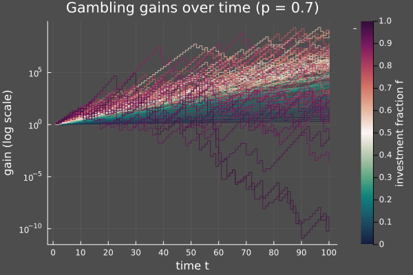
You clearly see that having $f$ very close to $1$ (violet paths) yield the absolute worst results, in practice. So what's the best value? It seems to fit somewhere inside the yellow-orange region –- that is, between 0.4 and 0.7.

The Kelly strategy

Kelly noticed that, if the number $n$ of epochs is large, the portion of winning bets should be close to $p$, that is we roughly have $S_n/n \approx p$ by the Law of Large Numbers. Consequenly,

$$R_n \approx ((1-f\ell) \gamma^{p})^n = [(1+fw)^p(1-f\ell)^q]^n.$$

Now you want to maximize this to get the optimal $f_{\mathrm{kelly}}$. This is equivalent to finding the max of

$$p\log(1+fw) + q\log(1-f\ell)$$

and after elementary manipulations the optimal fraction $f_{\mathrm{kelly}}$ is

$$\begin{aligned}f_{\mathrm{kelly}} = \frac{p}{\ell} - \frac{q}{w} .\end{aligned}$$

Here it should be understood that if $f_{\mathrm{kelly}}$ is negative or greater than $1$, we clip it to 0 or 1. For most cases though, $f_{\mathrm{kelly}}$ will be between $0$ and $1$. For instance if $a=b=1$ it is equal to $p-q = 2p-1$.

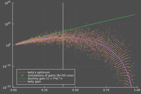
Here's an illustration with $p=0.7$. The purple line corresponds to the mean gain predicted by Kelly and it's maximized for $f=p-q=0.4$. Orange dots are samples for this specific $f$.

Is there a paradox?

We adopted two plans for finding the $f$ maximizing the final wealth, but they don't match. The no-brain approach seems theoretically sound while in the Kelly approach, the approximation (5) might seem suspicious; but the numerics clearly show that for $f=p-q=0.4$ you alwost always end up with a greater wealth than with $f$ close to 1. Kelly's approach is justified by arguing that Kelly does not optimize the same objective as the nobrainer; indeed, Kelly rigorously maximizes the logarithm of the gain:

$$\begin{aligned} \mathbb{E}[\log(R_n)] &= n\log(1-f\ell)+ \mathbb{E}[S_n\log(1+fw)/(1-f\ell)] \\ &=n\log(1-f\ell)+ np \log(1+fw)/(1-f\ell) \\ &= n [p\log(1+fw) + q\log(1-f\ell)] \end{aligned}$$

which is exactly $n$ times (6). How would one justify maximizing the logarithm of the wealth instead of the wealth? Well, one potential justification is with utility functions, that thing from economy –- but this is indeed not a good justification.

Utility functions

If you win 1000€ when you have only, say, 1000€ in savings, it's a lot; but if you win 1000€ when you already have 1000000€, it means almost nothing to you. The happiness you get for each extra dollar increases less and less; in other words, the utility (I hate the jargon of economists) you get is concave. Your utility function could very well be logarithmic, and the Kelly criterion would tell you how to maximize your logarithmic utility function.

This interpretation is the one put forward by SBF in his famous thread, and it is mostly irrelevant, as already noted by Kelly himself.

The twist is that with utility functions, you could justify any a priori strategy $f$. They're not a good tool for understanding people's behaviour or elaborating investment strategies. You can even exercice yourself by finding, for any fixed $f \in [0,1]$, a concave utility function $\varphi$ such that the maximum expected utility $\mathbb{E}[\varphi(R_n)]$ is attained at $f$.

That's more or less how SBF justified his crazy over-leverage strategy, by saying that his own utility function was closer to linear ($f=f_{\mathrm{degen}})$ than logarithmic ($f = f_{\mathrm{kelly}})$. In his paper, Kelly actually argues that rather than taking his criterion as the best possible, we should take it as an upper limit above which it should be completely irrational to go. SBF, on the other hand, used this analysis to justify all-or-nothing strategies which resulted in, well, quite bad an outcome.

The Kelly criterion is a an empirical rule

Actually, the Kelly criterion relies on empirical gain maximization.

In a more realistic setting where you could play a Kelly gambling game, you wouldn't know $p$, but you probably would have access to a history of data from past players; that is, you would have a long historical series $x_1, \dotsc, x_N$ where $x_i$ is the outcome of the $i$-th bet (win or lose). If you had played this game at these times, with an $f$-fixed fraction strategy, you would exactly have won

$$\hat{R}_N(f) = (1 + fa)^{s_N}(1 - fb)^{N-s_N}$$

where $s_N = x_1 + \dotsb + x_N$ is the total number of past wins. But then, the optimal $\hat{f}$ which maximizes this empirical gain would precisely be (do the maths): 

$$\hat{f} = \frac{s_N}{N\ell} - \frac{N-s_N}{Nw} = \frac{\hat{p}}{\ell} - \frac{\hat{q}}{w}$$

with $\hat{p}=s_N/N,\hat{q} = 1 - \hat{p}$ the natural estimators for $p$ and $q=1-p$. And if $N$ is large enough, the LLN gives us $\hat{p}\approx p$ and $\hat{f}\approx f_{\mathrm{kelly}}$.

Beyond gambling

The nice part about the Kelly criterion as an empirical gain maximization rule is that you can apply it well beyond the simplistic win/lose framework. For example, should you invest in Stock, you have at your disposition a time series of returns $r_t$ for $t=1, \dotsc, T$; say, $r_t$ is the daily return of some stock. Starting with 1, your gain with an $f$-fixed fraction strategy would have been $\prod_{t=1}^T (1+fr_t)$. Your best fixed-fraction strategy would then maximize the function

$$\hat{R}(f) = \sum_{t=1}^T \ln(1 + fr_t).$$

Of course, this is interesting only when some returns $r_t$ can be extreme. If $r_t$ is close to 0, the above function is just approximated by $fs$ where $s=\sum r_t$ since $\ln(1+u)\approx u$, and the optimal $f$ would always be $0$ if $s<0$ and 1 otherwise.

Concluding remarks 

1. Always look for geometric returns, not arithmetic.

2. The Kelly criterion is over-simplistic. Quantitative investment books are full of variants.

3. If you justify your actions by your utility function, chances are you're just out of control.

4. Don't invest in crypto now

Notes

^[1] the « full degen » strategy, as Eruine says