🏋🏼 Heavy tails III: Kesten's theorem

Motivation: ARCH models

In 2003, Robert F. Engle won the Nobel prize in economy for his innovative methods in time-series analysis; to put it sharply, Engle introduced ARCH models into economics. In his seminal 1982 paper (30k+ citations), he wanted to model the time-series $(y_t)$ representing the inflation in the UK. Most previous models used a simple autoregressive model of the form $y_{t+1} = \alpha y_t + \varepsilon_t$, where $\varepsilon_t$ is an external Gaussian noise with variance $\sigma^2$ and $\alpha<1$ a "forgetting" parameter. The problem with these models is that the variance of the inflation at time $t+1$ knowing the inflation at time $t$, that is $\mathrm{Var}(y_{t+1}|y_t)$, is simply the variance of $\mathrm{Var}(\varepsilon_t)=\sigma^2$, which does not depend on $y_t$.

Engle wanted a model where the conditional variance would depend on $y_t$: there are good reasons to think that volatility is sticky. The model he came up with (equations (1)-(3) in his paper) is simply

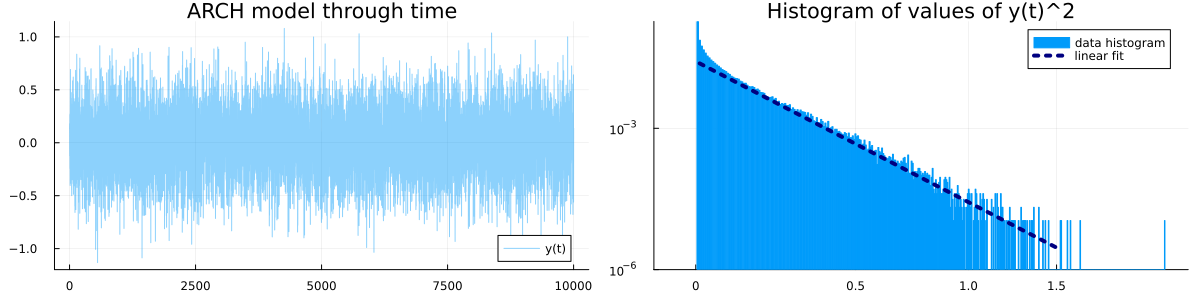
In other words, the variance of $y_{t+1}$ given $y_t$ is $\alpha + \beta y_t^2$. This is the simplest of Auto-Regressive Conditionally Heteroscedastic (ARCH) models. Upon squaring everything in (1), the equation becomes

This is a linear recursion in $y_t^2$. In the paper, Engle introduced a few variations and crafted statistical methods to estimate the parameters and their significance.

If $y_t^2$ converges in distribution towards a random variable $Y$, then (2) shows that $Y$ and $\alpha \varepsilon^2 + \beta \varepsilon^2 Y$ must have the same probability distribution, where $\varepsilon$ is an $\mathscr{N}(0,\sigma^2)$, independent of $Y$. This is an instance of a very general kind of equations, called affine distributional equations: they are equations of the form

where $A,B$ are random variables independent of $Y$. It turns out that these equations are generally impossible to solve. However, a theorem of Harry Kesten states, perhaps not so intuitively, that the law of any solution must have a heavy tail: in contrast with, say, Gaussian distributions, for which taking extremely large values (« shocks ») has an exponentially small probability, heavy-tailed distributions can take large values with polynomially small probability, which is… not so rare at all!

Here is a small simulation over $10^6$ periods of time and parameters $\alpha=0.1, \beta=1, \sigma = 0.1$. The histogram indicates that $y(t)$ seems to have heavy tails, that is, the probability of observing a unusually large value is polynomially small (and not exponentially small).

Kesten's theorems

From now on, we'll study the solutions of the equation

where $X$ is a random variable over $\mathbb{R}^d$, $A$ is a random matrix and $B$ a random vector, both independent of $X$. The goal is to present Kesten's theorem, which states that on certain conditions on $A$ and $B$, the solution $X$ must have heavy tails; that is, $\mathbb{P}(X>x)$ decreases polynomially fast, and not exponentially fast as for Gaussian variables. This result is somehow mind-blowing in its precision, since we have access to the exact tail exponent.

A full, rigorous proof would be packed with technicalities; I'll only show a simili-proof in dimension $1$, which, although not being complete, was sufficiently clear and idea-driven to convince me that Kesten's result holds. I'm also including a simili-proof of the Renewal theorem, which might be of independent interest.

One-dimensional case

For simplicity, we restrict to the case where $A,B$ are independant and have a density with respect to the Lebesgue measure. In general, it is not obvious that solutions to (4) exist, but a former result by Kesten states that it is the case if $\mathbb{E}[\ln |A|]<\infty$.

Sketch of proof in the 1d case

I'll only sketch the proof ideas in the subcase of (i) where in addition, $B$ is nonnegative. In this case, we can safely assume that $X$ is nonnegative by conditionning over the set $\{X>0\}$. We set $f(x) = e^{sx}\mathbb{P}(X > e^x)$; our final goal is to prove that $f(x)$ converges towards some constant when $x\to+\infty$, the $-\infty$ case being identical.

The recursion (4) shows that $f(x) = e^{sx}\mathbb{P}(AX + B > e^x)$. However, if $x$ is very large, we could guess that $\mathbb{P}(AX + B > e^x)$ is close to $\mathbb{P}(AX > e^x)$. This is the origin of the first trick of the proof, which is to artificially write

Let us note $g$ the first term on the right:

For the second term, we can express it in terms of $f$ by using $\mathbb{E}[A^s]=1$:

Now, here comes the second trick: the change of measure. We assumed that $\mathbb{E}[A^s]=1$, hence we can define a probability distribution by $\mathbb{E}_s[\varphi] = \mathbb{E}[A^s \varphi]$, and the expression above becomes $\mathbb{E}_s[f(x- \ln A)]$. Overall, we obtain that $f$ is a solution of the following equation: 

If $\mu_s$ is the density of $\log A$ under the measure $\mathbb{P}_s$, this equation becomes $f(x) = g(x) + f\star \mu(x)$ where $\star$ denotes the convolution operator. Such equations are called convolution equations and they can be studied using classical probability theory. The main result of Renewal Theory, exposed later below, shows that

• if $g$ is « directly Riemann integrable »; 

• and if $\mathbb{E}_s[\ln A]>0$, which is the same thing as $\mathbb{E}[A^s \ln(A)]>0$;

then there is only one solution to this equation, and more crucially it satisfies

If $\mathbb{E}[A^s \ln A]>0$, as we assumed, then $c>0$, because $g$ is a nonzero positive function so its integral is nonzero. Consequently,

This is equivalent to $\mathbb{P}(X>x) \sim cx^{-s}$, as requested. There is, however, a serious catch: to apply the main Renewal theorem we need to check the two conditions listed above. The second one is nothing but an assumption. However, the first one needs $g$ to be "directly Riemann integrable", which is indeed very difficult to check. I won't do this part at all^[1].

Multi-dimensional case

In the multi-dimensional case, a similar theorem holds. One can find in the litterature a host of different settings regarding the random matrix $A$ and the random vector $B$; for simplicity I'll stick to the case where $A$ is positive definite almost surely, $B$ has all entries nonnegative almost surely, and $A,B$ have densities with respect to the Lebesgue measure. The multi-dimensional analogue of $\mathbb{E}[|A|^s]$ will now be

where $\Vert M \Vert$ is the operator norm. We also introduce the Lyapounov exponent, which is the equivalent of $\mathbb{E}[\ln |A|]$:

The proof is much more technical without any new ideas.

Renewal theory in less than one page

Let $\mu$ be a continuous probability distribution on $\mathbb{R}_+$. Our goal is to show how renewal theory can be used to study convolution equations, represent their solutions with a probabilistic model, and draw consequences on their asymptotic behaviour. We are interested in finding $f$ such that

where $g$ is some function. Noting $f\star \mu(x) = \int f(x-u)\mu(du)$, we recognize a convolution between the function $f$ and the measure $\mu$, and the equation is simply $f - \mu \star f = g$. Upon noting $U$ a random variable with distribution $\mu$, we can also represent this equation as

But if this equation is satisfied for some $f$, then plugging it into $f(x-U)$ yields

and so on, with $U,U',U''...$ iid copies of $U$. The following theorem follows by iterating this trick infinitely.

The name "renewal process" comes from the fact that the $S_n$ are considered as occurence times of events. The $U_i$ are thus waiting times between the events. Renewal theory is interested in processes like $N_t=$ the number of events before time $t$.

It is quite rare that the representation theorem yields the explicit solution $f$. One would need to compute the expectation of the series, which is most cases can be tedious. But this representation gives access to the whole toolbox of limit theorems in probability, and in particular, laws of large numbers, which translate into exact asymptotics for $f$. That's the key renewal theorem.

• « Directly Riemann integrable » is the true equivalent of « Riemann integrable », but for functions defined over $\mathbb{R}$ or the half-line. It states that the Riemann sums over the whole domain (they are indeed series, not sums, in contrast with the classical definition) converge toward the same limit.

• The intuition is pretty clear. In Blackwell's version, $\mathbb{E}[N_{t+a} - N_t]$ is nothing but the number of $S_n$ in the interval $[t,t+a]$. If the size of each jump is roughly $\mathbb{E}[U]$ then the number of jumps in this interval should be proportional to the length of the interval divided by $\mathbb{E}[U]$; Blackwell's theorem says that this is true when $t\to\infty$. Note that in this case $g=\mathbf{1}_[-a,0]$ and $\int g(u)du = a$.

• By linearity, Blackwell's version extends to (22) at least for piecewise constant functions with bounded support. To extend to wider functions, a limiting argument is needed, and this is where direct Riemann integrability comes into play.

• We can very well have $\mathbb{E}[U] = \infty$ in this theorem but for simplicity I'll stick to the finite case.

• The theorem is also valid when $U$ is not necessarily positive, but on the condition that $\mathbb{E}[U]>0$. This version is due to Athreya et al. (1978).

• A full, readable proof can be found in Asmussen's book. I'll probably write a note on this topic, some day.

References

• Kesten's original paper, really hard to read.

• Goldie's paper, which both simplified and generalized Kesten's proof (the proof in this note is Goldie's). Hard to read too.

• ARCH models by Engle.

• An excellent book on the topic by Buraczewski, Damek and Mikosch. This is where I learned the proof of Kesten's theorem. It's very well written.

• Another excellent book with a chapter on the Renewal Theorem, by Asmussen.