Waves on donuts
August 2021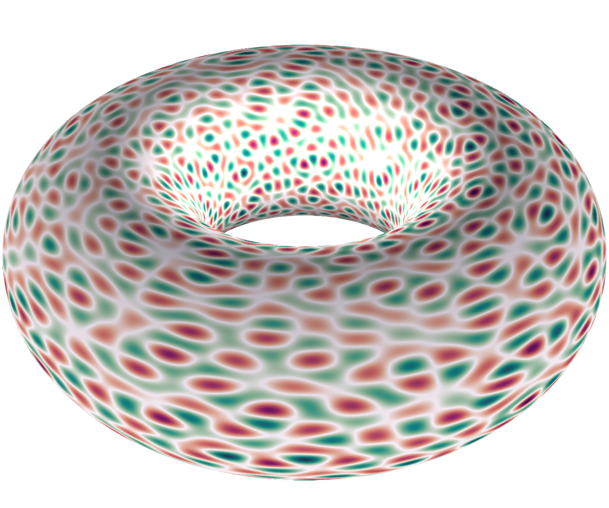
The Laplace eigenequation on a sphere, a torus, or any Riemannian manifold is
where is the Laplace operator on the manifold. On the torus , this equation is well understood and the goal of this note is simply to plot the typical solutions – they look like the donut above.
The only values for which there are solutions to (1) are multiples of ,
where is an integer that can itself be written as the sum of two squares, ie . The function is easily seen to be an eigenfunction: indeed,
Sum of squares
Determining if an integer satisfies this property, to be the sum of two squares, is an old problem with a long history - it dates back to Diophante. Fermat gave the first characterization of such prime numbers. The general theorem is as follows.
An integer can be written as the sum of two squares if and only if, in its prime decomposition, the primes with of the form have an odd power. If it is the case, then the number of ways to write as a sum of two squares is given by
where is the number of divisors of , not necessarily primes, which are congruent to modulo .
For example, ; it has exactly four divisors , two of which are congruent to 1 modulo 4, two others to 2. Consequently, and and . These "sum-of-squares-representations" of 10 are
Here is a little function for generating all these representations (it is by no means optimized in any way):
function SOSrep(n::Int)
    """ Returns the list of Sum-Of-Squares representations.
    Returns an empty list if there are none. """
    square_reps = []
    for i in 1:sqrt(n)-1
        if isinteger(sqrt(n - i^2))
            j = sqrt(n - i^2)
            append!(square_reps,  [[i,j], [i,-j], [j,i], [j,-i]])
        end
    end
    if isinteger(sqrt(n))
        j = sqrt(n)
        append!(square_reps, [[0,j], [0, -j], [j, 0], [-j, 0]])
    end
    return square_reps
end
Random arithmetic waves
Let us go back to the Laplace equation (1). Let be an integer that can be written as a sum of squares and let be the associated eigenvalue. Then, the subspace of solutions of (1) has dimensions , the number of ways to write as a sum of squares discussed above. Let be the set of couples with ; then, a basis of is given by the elementary functions
and the solutions of (1) are all the linear combinations of these functions, namely the functions of the form
where are complex numbers. What we call random arithmetic waves are random elements of obtained by choosing the to be iid standard complex Gaussian variables[1]. The resulting random function is a random Gaussian field; it can be viewed as a typical element of , and there is a vast litterature on its behaviour. Usually, it is more natural to study real Gaussian fields, and for this we have to ensure that is real by enforcing some minor constraints on the : we simply ask that (complex conjugate).
We generate a random arithmetic wave with the following function:
function generate_RAW(n::Int)
    Λ = SOSrep(n)
    if isempty(Λ)
        return nothing
    else
        E = [(x,y) -> exp(2im*pi*(λ[1]*x + λ[2]*y)) for λ in Λ] #exponentials
        X = [randn() + 1im*randn() for λ in Λ]
        f(x,y) = sum(real(X.*[e(x,y) for e in E])) / sqrt(length(Λ))
        return f
    end
end
Let us generate some arithmetic wave; most numbers have very few sum-of-squares representations (0,4 or 8), but has 16 of them.
f = generate_RAW(85)Also, 71825 has 68 square representations, and 801125 has 124, which is a lot.
Some code
A torus can be parametrized with two coordinates by the following formulas:
X(θ, φ) = (2 + cos(θ)) * cos(φ)
Y(θ, φ) = (2 + cos(θ)) * sin(φ)
Z(θ, φ) = sin(θ)
And now, let's use Julia's GLMakie, which is Makie's backend for GPU 2d and 3d plotting, to see how looks like. We're going to draw a mesh of with a mesh-size of .
ε = 0.01
t = 0:ε:2π+ε ; u = 0:ε:2π+ε
x = [X(θ, φ) for θ in t, φ in u]
y = [Y(θ, φ) for θ in t, φ in u]
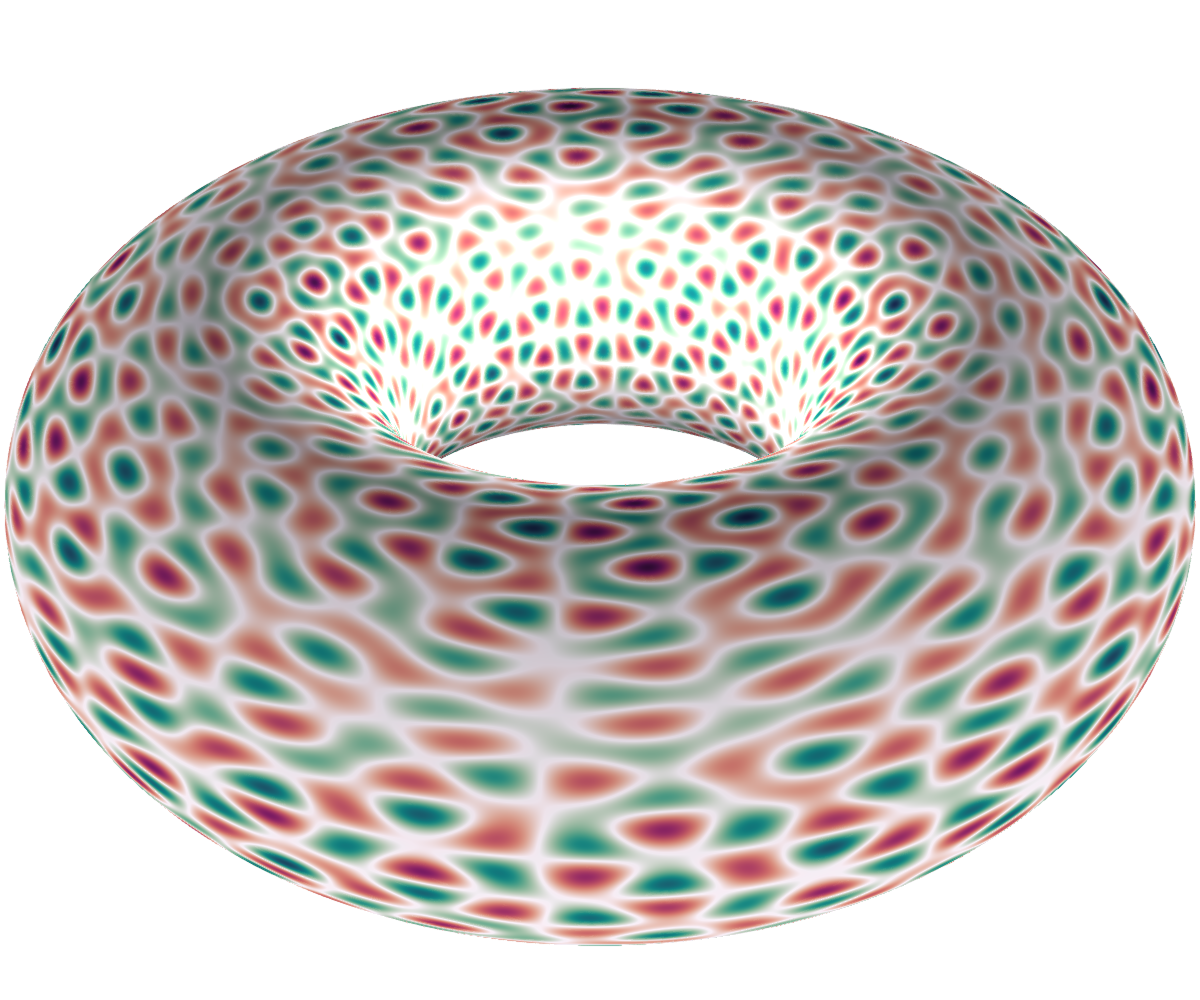
z = [Z(θ, φ) for θ in t, φ in u]For each mesh point , we'll color the corresponding point of the torus, , with a color representing the field .
using GLMakie

field = [f(θ, φ) for θ in t, φ in u]
fig, ax, pltobj = surface(x, y, z, color = field,
        colormap = :vik,
        lightposition = Vec3f0(0, 0, 0.8),
        ambient = Vec3f0(0.6, 0.6, 0.6),
        backlight = 5f0,
        show_axis = false)

cbar = Colorbar(fig, pltobj,
        height = Relative(0.4), width = 10 )

fig[1,2] = cbar #hide
set_theme!(figure_padding = 0)#hide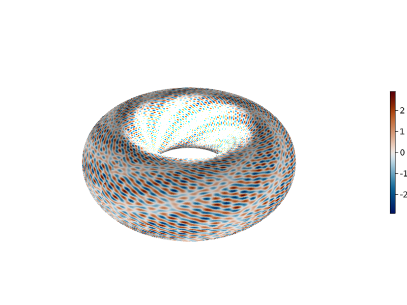
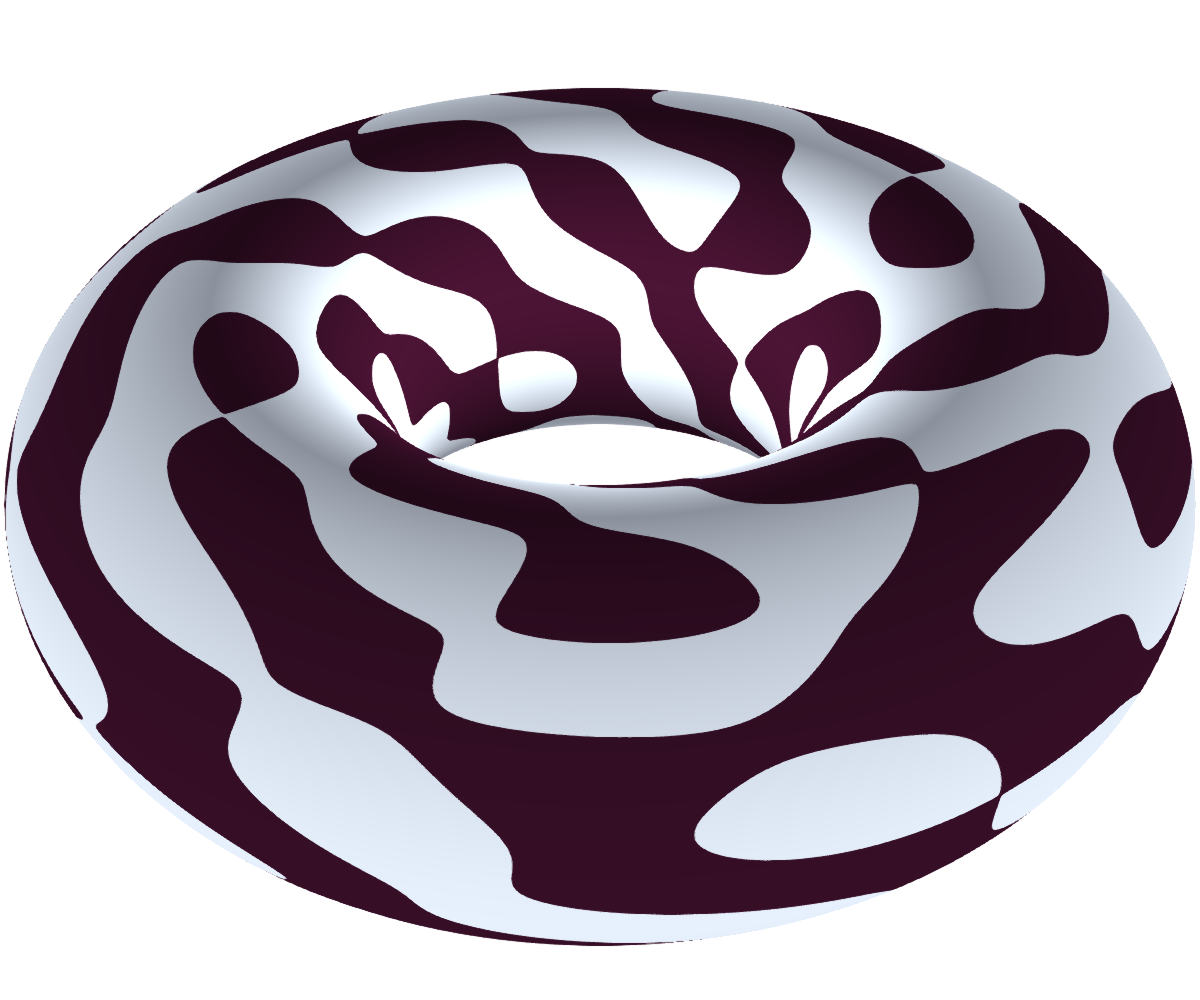
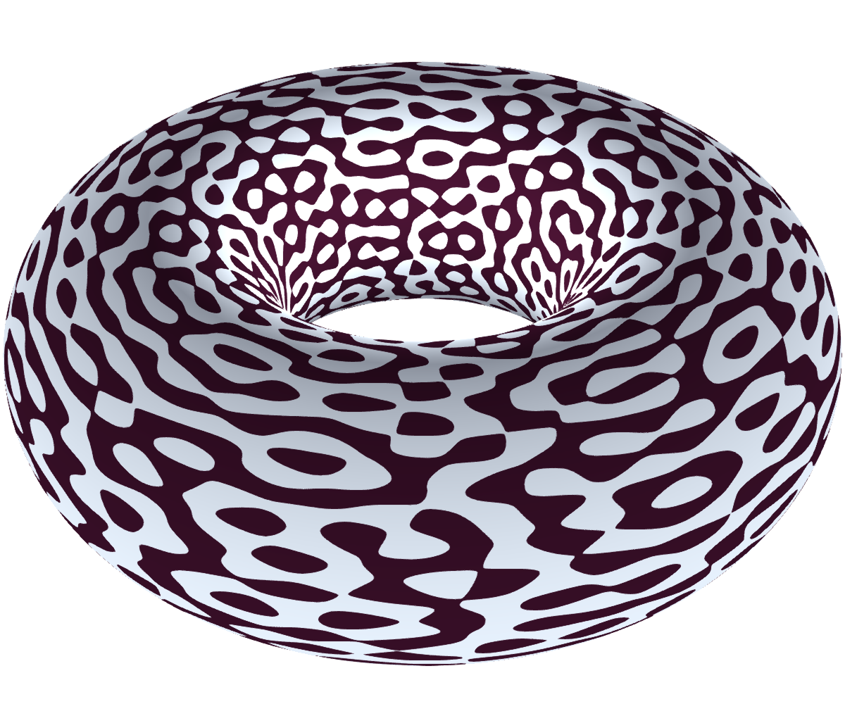
Instead of plotting each color, we can only plot the sign of , black if positive and white if negative. The set of points of the torus where is zero is called the nodal line while the sets and are called nodal sets.
signs = [x > 0 ? 0 : 1 for x in field]
fig2, ax2, pltobj2 = surface(x, y, z, color = signs,
        colormap = :ice,
        lightposition = Vec3f0(0, 0, 0.8),
        ambient = Vec3f0(0.6, 0.6, 0.6),
        backlight = 5f0,
        show_axis = false)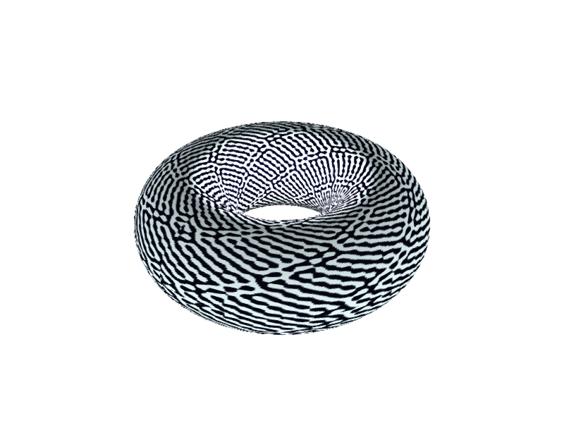
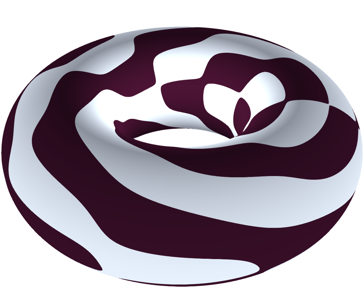
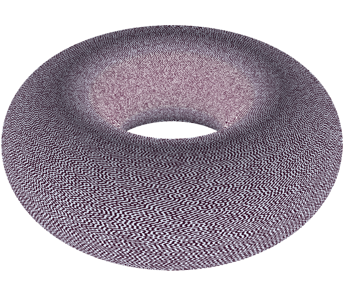
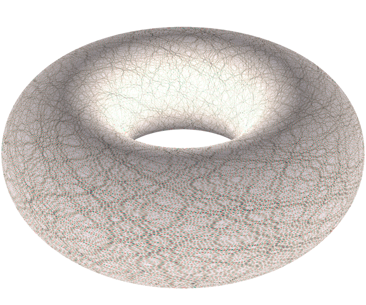
With a few processing and computational power, one can get much detailed pictures !
Gallery
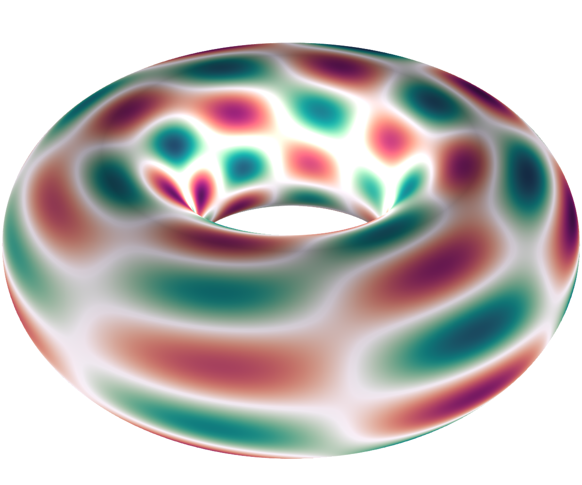
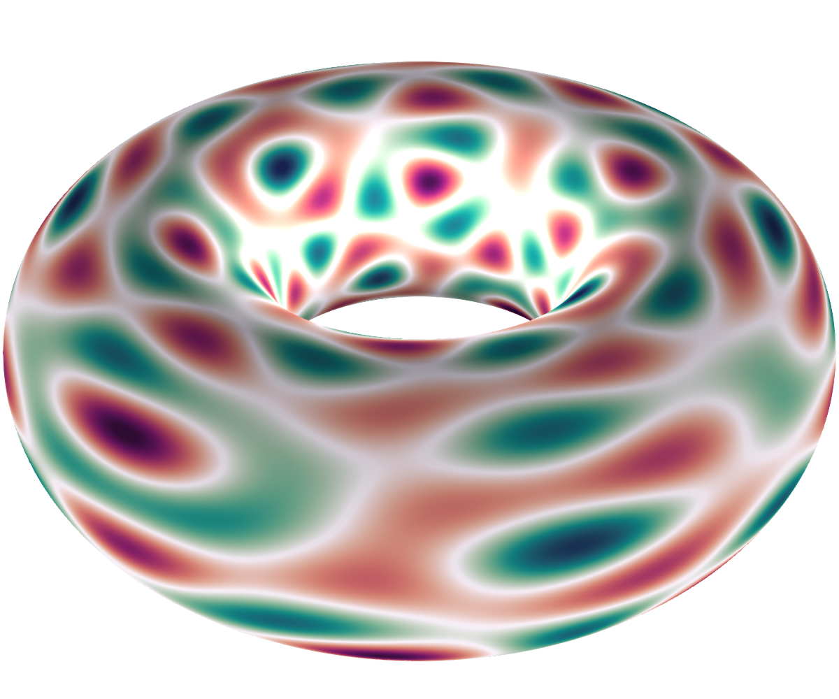
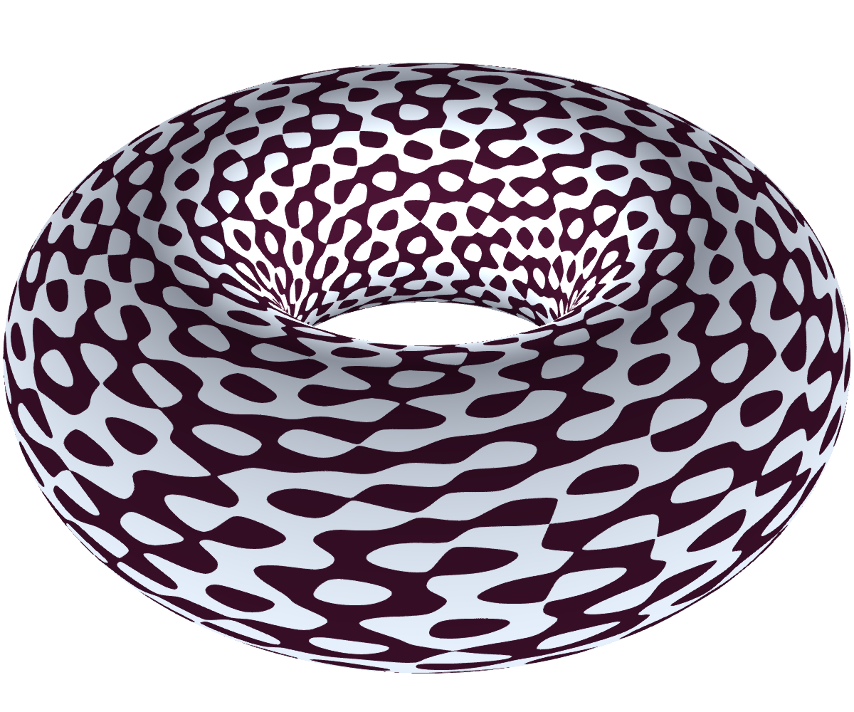
Here are some pictures of realizations of various arithmetic waves associated with different values of . The left picture is the nodal set ( is dark), while the right one is a heatmap: white is close to zero, red is negative and green is positive. Note that the left and right picture do not correspond to the same realization of the wave (I'll update this soon to see the same realization).
You can use these pictures if you want, but if so please mention this page.
, dimension 8
, dimension 12
, dimension 16
, dimension 28
, dimension 64
Notes and references
The paper Nodal length fluctuations for RAW by Krishnapur et al. studies the length of the nodal lines of random arithmetic waves, while this paper by Rudnick and Wigman studies the volume of nodal sets. See the references in these papers for more litterature on the topic. For spherical random waves or plane random waves, Dimitry Belyaev has some nice pictures on his website.
Also, a gallery of Makie plots which turned out to be quite useful.
Extra pictures on request.
| [1] | Usually there is also a normalization by , but it's not important. |