🏋🏼 Heavy tails I: extremes events and randomness

November 2023

The famous Pareto principle states that, when many independent sources contribute to a quantitative phenomenon, roughly 80% of the total originates from 20% of the sources: 80% of the wealth is owned by (less than) 20% of the people, you wear the same 20% of your wardrobe 80% of the time, 20% of your efforts are responsible for 80% of your grades, 80% of your website traffic comes from 20% of your content, etc.

This phenomenon mostly comes from a severe imbalance of the underlying probability distribution: for each sample, there is a not-so-small probability of this sample being unusually large. This is what we call heavy tails. In this post, we'll give a mathematical definition, a few examples, and show how they lead to Pareto-like principles.

The tail distribution of a random variable
Examples of heavy-tailed densities
The Lorenz curve of heavy-tailed distributions
References

The tail distribution of a random variable

If $X$ is a random number, the tail of its distribution is the probability of $X$ taking large values: $G(x)=\mathbb{P}(X>x)$ . Of course, this function is decreasing in $x$ ; the question is, how fast?

Light tails

Some distributions from classical probability have tails which decrease quickly toward zero. It is the case for Gaussian random variables: a classical equivalent shows that if $X \sim \mathscr{N}(0,1)$ , then when $x$ is very large^[1]

\mathbb{P}(X>x) \sim \frac{e^{-x^2/2}}{x\sqrt{2\pi}}.

This probability is overwhelmingly small. For example, $\mathbb{P}(X>5)$ is already smaller than $0.00001\%$ . It means that if you draw $10000$ samples from $X$ the probability of having one of those samples greater than $5$ is approximately $0.3\%$ . That's possible, but very rare.

Heavy tails

A distribution is heavy-tailed when $\mathbb{P}(X>x)$ does not decay as fast as $e^{-x^2}$ or even $e^{-x}$ , but rather like inverses of polynomials: $1/x$ or $1/x^2$ for example. That's the case with the ratio of two standard Gaussian variables $X/Y$ , whose density is $1/(\pi(1+x^2))$ . For this distribution called the Cauchy distribution^[2], a direct computation gives

\mathbb{P}(X>x) = \frac{1}{2} - \frac{\mathrm{arctan}(x)}{\pi} \sim \frac{1}{\pi x}.

This decays very slowly. For example $\mathbb{P}(X>5)\approx 1/5\pi \approx 6\%$ , which means that if you draw as few as 100 samples from $X$ then you will see one of the samples larger than 5 with probability $99.8\%$ . That's a very different behaviour than the preceding Gaussian example.

Mathematically, we say that a distribution is heavy-tailed if $\mathbb{P}(X>x)$ is asymptotically comparable to $1/x^s$ for some $s$ . By "asymptotically comparable", we mean that terms like $\log(x)$ should not count. There is a class of functions, called slowly varying, encompassing this: they are all the functions which are essentially somewhere between constant and logarithmic. Just forget about this technical point: for the rest of the note, think of "regularly varying" as "almost constant". I will keep this denomination.

Definition. A distribution is heavy-tailed if there is an essentially constant function

c

and an index

s>0

such that

\mathbb{P}(X>x) = \frac{c(x)}{x^s}.

The same definition holds for $x\to -\infty$ .

Densities

If $X$ has a density $f$ , then one can generally see the heavy-tail of $X$ in the asymptotics of $f$ . Roughly speaking, if for example $f(x) \approx c / x^{s+1}$ when $x$ is large, then $\mathbb{P}(X > x) \approx c\int_x^\infty x^{-s-1}dx = c' x^{-s}$ , so $X$ is heavy-tailed with index $s$ . Most of our following examples will have densities.

Log-scales

On the left, you see the two densities mentioned above: Gaussian and Cauchy. On classical plots like this, it is almost impossible to see if something is heavy-tailed or not. The orange curve seems to go to zero slower than the blue one, but at which rate? This is why, when it comes to heavy tails, log-scales on plots are ubiquitous. The plot on the middle is the same as the one on the left, but with a log-scale on the y-axis; and on the right, both axes have a log-scale.

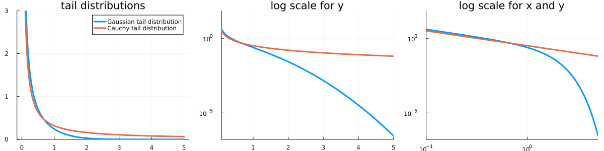
In fact, if $X$ has a density $f$ , then discerning by bare visual inspection if $f(x)$ decays to zero rather polynomially or exponentially is almost impossible. But on a log-log scale,

if $f(x)\approx c/x^r$ we have $\log f(x) \approx \log(c) - r \log(x)$ : on a log-log plot, this is a linear relation ( $y=ax+b$ ).
while if $f(x)$ is (say) exponential, $f(x) \approx ce^{-x^r}$ , then $\log f(x) \approx \log(c) - x^r = \log(c) - e^{r\log (x)}$ . On a log-log plot, this is an exponential relation ( $y = ae^{bx} + c$ ).

This is why most plots you will see on this topic are on log-scales or log-log scales.

Examples of heavy-tailed densities

The Power-Law, or Pareto distribution

The most basic and important example of a heavy-tailed distribution is the Pareto one. It is directly parametrized by its index $s>0$ and its density is given by

\rho_s(x) = \frac{s\mathbf{1}_{x>1}}{x^{s+1}}.

I started the distribution at 1, but some people add its starting point as a second parameter. It's really not important. The Pareto law is often denoted $\mathrm{PL}(s)$ .

Other heavy-tailed densities

The Fréchet distribution has CDF and PDF

F_s(x) = e^{-x^{-s}} \qquad \rho_s(x) = \frac{s\mathbf{1}_{x>0}}{x^{1+s}}e^{-x^{-s}}.

Closely related is the Inverse Gamma distribution,with

F_{\lambda, s}(x) = \frac{\Gamma(s, \lambda/x)}{\Gamma(s)} \qquad \rho_{\lambda,s}(x) = \frac{\lambda^s}{\Gamma(s)}\frac{\mathbf{1}_{x>0}}{x^{s+1}}e^{-\frac{\lambda}{x}}.

When $s=1/2$ , this is often called a Lévy distribution. It is a special case of the $\alpha$ -stable distributions, which encompasses the Cauchy distribution. There is also the Burr distribution (of type XII), with density

f(x) = \frac{ckx^{c-1}}{(1+x^c)^{k+1}}.

A shortlist of mechanisms leading to heavy tails.

There are many survey papers on why heavy tails do appear in the real world, like Newman's one. In general, the most ubiquitous cases are the following ones:

simple transforms (like inverses or exponentials) of distributions. For example, the inverse of a uniform random variable has a heavy tail with index $1$ .
Maxima of many independent random variables often converge (after proper normalization) towards heavy-tailed distributions. This is called the Fisher-Tippett-Gnedenko theorem. This is why many areas in applied statistics (insurance, lifetime estimation, flood predictions, etc) have to deal with heavy tailed distributions.
Any dynamic phenomenon where an growth rate is independent of the size leads to sizes which are exponentials of classical random variables. In economics, this is called Gibrat's law.
Random recursions of the form $X_{n+1} = A_n X_n + B_n$ often converge towards heavy-tailed distributions. This is a very deep result by Harry Kesten and I wrote a note on this topic.
The number of connections of nodes in a large network often follows a heavy-tailed distribution. This is notably the case for the Albert-Barabasi preferential attachment model.
Zipf's law is probably the most famous example. It says that the probability of a word appearing in a text is inversely proportional to its use rank: for example, the second most-used word ("of") is two times less frequent than the first one ("the").

The Lorenz curve of heavy-tailed distributions

Now, let us see how heavy tails are the kind of distributions accountable for imbalances like the 80-20 principle. In general, we measure such imbalances using the Lorenz curve: this curves gives the amount of mass "produced" by the $t$ -th quantile of a probability distribution. By "mass", we mean the mathematical expectation. The correct definition of the Lorenz curve is the curve joining all points $(F(x), M(x))$ for all $x$ , where $F(x) = \mathbb{P}(X < x)$ is the proportion of samples below level $x$ , and

M(x) = \frac{\mathbb{E}[X\mathbf{1}_{X < x}]}{\mathbb{E}[X]}

is the proportion of the total mean $\mathbb{E}[X]$ coming from samples below $x$ . This is the same curve as $(t, M(q(t))$ where $q = F^{-1}$ is the quantile function.

For Pareto distributions, we have $F(x) = 1 - t^{-s}$ hence $q(t) = (1-t)^{-1/s}$ . On the other hand $\mathbb{E}[X] = s/(s-1)$ and

\mathbb{E}[X\mathbf{1}_{X < x}] = s\int_1^x \frac{y}{y^{s+1}} dy = \frac{s}{s-1}\left(1 - \frac{1}{x^{1-s}}\right)

so that $M(x) = 1 - x^{s-1}$ . A mere computation gives the following picture.

Mass imbalance in heavy-tails.

The Lorenz curve of a $\mathrm{PL}(s)$ is given by $t \mapsto 1 - (1 - t)^{1 - \frac{1}{s}}$ .
The quantile contributing the last 80% of the total mass is given by $\mathfrak{q}_{0.8}(s) = 1 - 0.8^{s/(s-1)}$ . I call this quantile the "Pareto Index" in the next picture below.
Pareto's "80-20 principle" corresponds to $s=1.16$ .

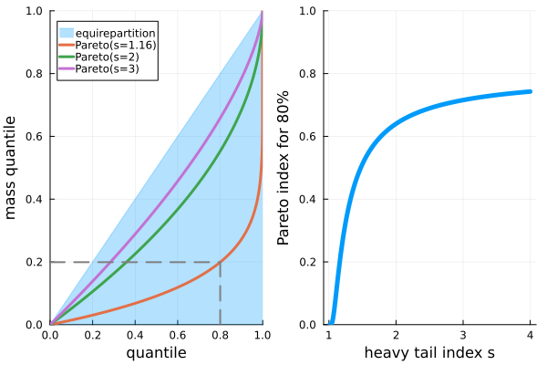
As shown with the dotted lines, the tail-index which seems to fit the 80-20 principle is $s=1.16$ . For this index (as for any index $1 < s < 2$ ), the Pareto distribution has a finite mean but no finite variance. For general heavy-tailed distributions, we would have the same kind of pictures, with really convex Lorenz curves. Of course, since the distribution becomes more and more heavy-tailed when $s$ is closer and closer to 1, these curves are less convex when $s$ increases.

In general, estimating the heavy-tail index $s$ is a difficult task. I have a note on this topic where I describe the Hill estimator.

References

The manual Fundamentals of heavy tails is simply the best book out there on heavy tails.
The book Fooled by Randomness, written by the unsufferable Nassim Nicholas Taleb, is a very good book on maths, stats, life, risk, finance, and randomness. As always with Taleb, shining pieces of wisdom are mixed with bad faith and purely idiotic stupidities – such books are the best books.
This paper by M. Newman is a gold mine for heavy-tail examples.
There's a self-improvement book on the 80/20 principle. Look at the cover: "the secret to achieving more with less", "the 80/20 principle is the cornerstone of results-based living", etc. These "books" are the equivalent of astrology or healing with stones, but marketed for overachieving young graduates starting a consulting carreer at McKinsey.

^[1] This estimate is very precise: the error is of order $e^{- x^2/2}/x^3$ , so as long as $x$ is greater than $5$ it is smaller than $0.00000001$ .

^[2] Indeed, $\arctan(x) + \arctan(1/x) = \pi/2$ and when $t=1/x$ is close to zero $\arctan(t)\sim \pi/2 - 1/t$ .